Metis Project Fletcher: Machine Learning with Tweets
May 29, 2015
For the fourth project of the Metis Data Science bootcamp, the only requirement was to include some kind of text processing. An intriguing aspect of text processing is the existence of two classes of methods, with little explanation of how they are related. Both classes require one to map documents to numerical vectors in a high-dimensional space (through a bag-of-words or Tf-Idf transformation), but one class uses purely algebraic methods whereas the other uses probabilistic tools:
-
Algebraic methods use cosine similarity to measure the semantic relatedness of two documents. Examples of such methods include K-Means and Latent Semantic Indexing (LSI).
-
Probabilistic methods start from a probabilistic model for the relationship between topics, documents, and words. Examples are Latent Dirichlet Allocation (LDA) and Hierarchical Dirichlet Process (HDP).
Suppose for example that we are asked to identify the topics discussed in a corpus of documents. One possible approach in the algebraic class is to cluster the documents with K-means, and identify topics with the top terms used in each cluster. In the probabilistic class one could use Latent Dirichlet Allocation (LDA) to find the underlying topics of the corpus, and then associate each document with the topic that has the highest probability for that document. In this way we obtain both topics and clusters from each method and we can compare them. This is what I attempted to do with a collection of tweets about yoga…
The Data: Tweets about Yoga
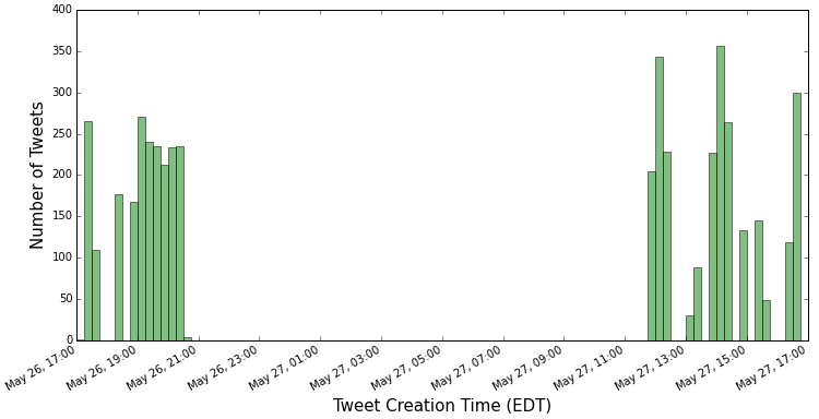
All tweets collected for this analysis were created in a 24-hour period starting at 17:00 (EDT) on May 26, 2015 (Figure 1). A total of 10,138 tweets with the keyword “yoga” were collected and stored in a Mongo database.
Using Python’s guess_language module, only tweets in English were kept, reducing the total to 7,244. After removing duplicates, 4,779 distinct tweets were left for analysis. To get some insight into the duplicates, I histogrammed in Figure 2 the number of “emissions” per tweet:
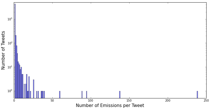
The tweet with the largest number of emissions (238) was an invitation:
"RT @mohitfreedom: #LetsStayfree and be #SultansOfStyle
at @IndianEmbassyUS Yoga Day celebrations of PM of #India
@narendramodi https://t.co/…"
The RT tag at the beginning signals that this is a retweet, and the ellipsis at the end indicates truncation (at least partly due to Twitter inserting the retweet tag).
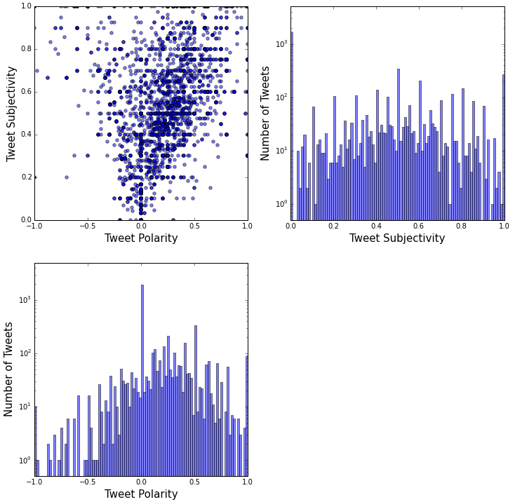
Python provides the TextBlob module to estimate the subjectivity and polarity of a text. Subjectivity is expressed on a scale from 0 to 1, whereas polarity goes from -1 to +1. Being akin to mood, polarity can be negative, neutral, or positive. Figure 3 shows a plot of subjectivity versus polarity for all 4,779 distinct tweets in the analysis. The distribution is skewed towards positive polarity, but positive tweets tend to be more subjective. Almost all tweets with zero subjectivity (1,656) have zero polarity (1,649).
To prepare the tweets for further processing I tokenized them, removed the “stopwords”, stemmed the remaining tokens (words), added n-gramsn-grams are contiguous sequences of n tokens. I chose to work with 1-grams, 2-grams, and 3-grams. , and removed n-grams that appear in more than a fraction max_df=0.80 of all tweets, or in less than a fraction min_df=0.01. Here is an example tweet and how it changes after each of these operations:
Original tweet: "I think I'm going to wear yoga pants to the office tomorrow."
After tokenization: ['i', 'think', 'i', "'m", 'going', 'to', 'wear', 'yoga', 'pants', 'to', 'the', 'office', 'tomorrow']
After removing stop words: ['think', 'going', 'wear', 'yoga', 'pants', 'office', 'tomorrow']
After stemming: ['think', 'go', 'wear', 'yoga', 'pant', 'offic', 'tomorrow']
After adding 2- and 3-grams: ['think', 'go', 'wear', 'yoga', 'pant', 'offic', 'tomorrow', 'think go', 'go wear', 'wear yoga', 'yoga pant', 'pant offic', 'offic tomorrow', 'think go wear', 'go wear yoga', 'wear yoga pant', 'yoga pant offic', 'pant offic tomorrow']
After removing n-grams with too large or too small a frequency: ['think', 'go', 'wear', 'pant', 'tomorrow', 'wear yoga', 'wear yoga pant', 'yoga pant']
Note how the word 'yoga' by itself disappears after the last step, due to its obviously high frequency in a corpus of tweets about yoga, but remains present as part of 2- and 3-grams. The distinct n-grams remaining in the corpus after this series of operations are referred to as “features”. The number of these features depends on the pruning parameters min_df and max_df as illustrated in Figure 4. As mentioned earlier I chose min_df=1% and max_df=80%, which yielded a total of 127 features.
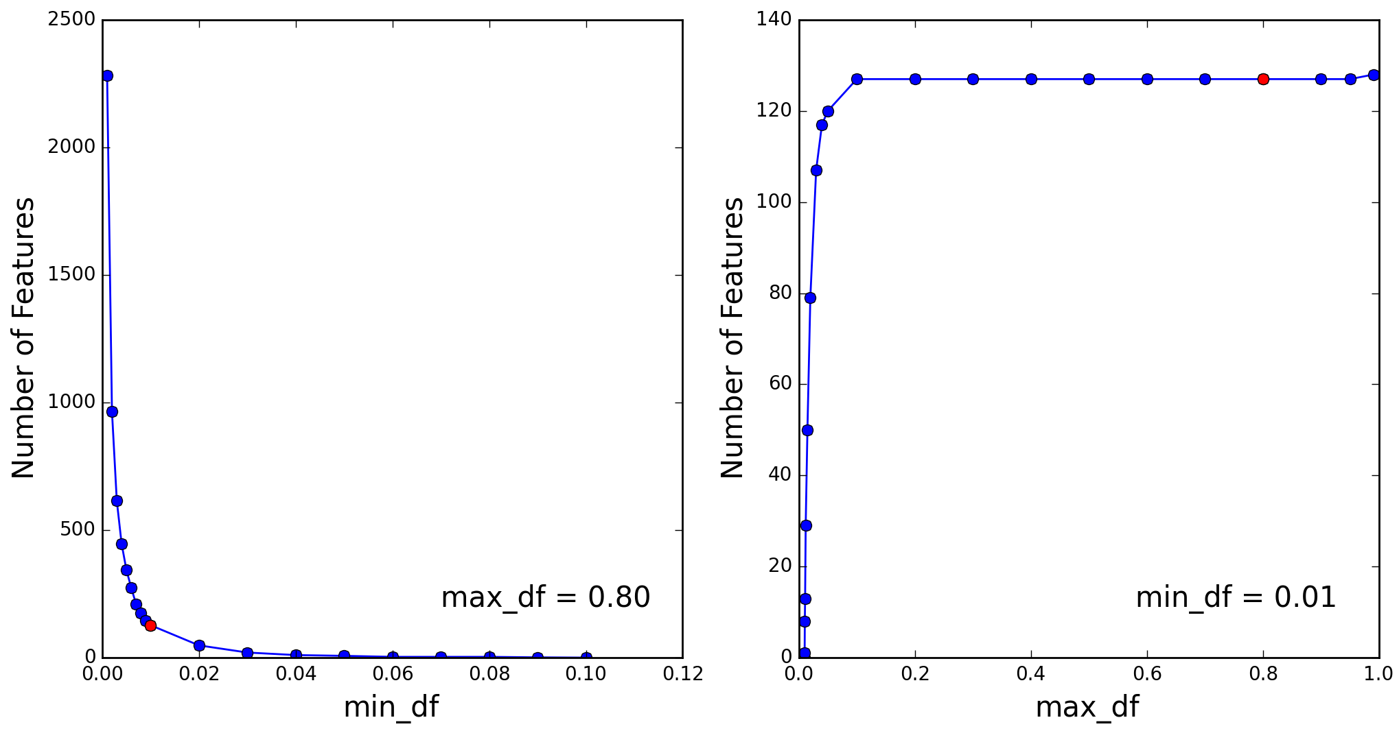
For the final pre-processing step I applied a Tf-Idf transformation. This converts the remaining n-grams within each tweet into numbers that reflect their frequency within the tweet and the inverse of their frequency within the entire corpus. Effectively, the original tweet corpus has been mapped into a 127 X 4,779 matrix of numbers, that is, into 4,779 vectors in a 127-dimensional space.
Multidimensional Scaling
How can we visualize such a high-dimensional space and the tweet vectors it contains? This is where a tool known as multidimensional scaling (MDS) comes in handy. MDS maps the 127 coordinates of each tweet into two coordinates than can be plotted on the page. The mapping attempts to preserve inter-tweet distances by minimizing the sum of squares of the differences between the distances in 127-dimensional space and the corresponding distances in 2-dimensional space:
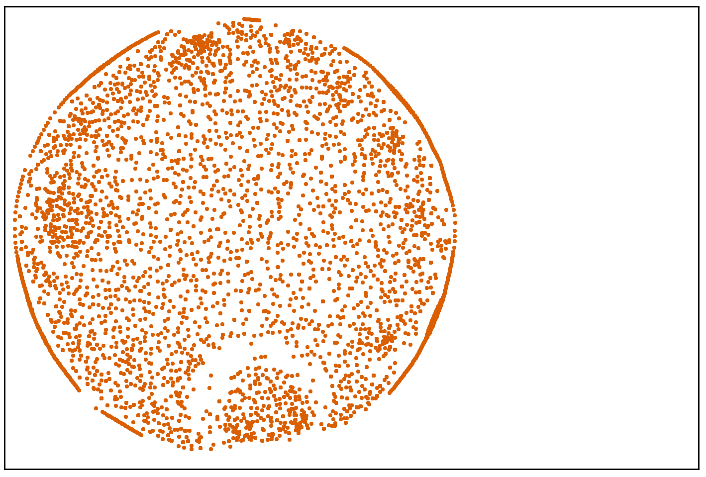
A careful look at Figure 5 reveals some structure. For example, just right of bottom center is a cluster of dots separated from the rest by a semicircular gap. Two additional clusters can be discerned near the border on the left and upper left. Before trying to interpret these clusters it is helpful to examine how well distances in 2-D space correlate with true distances in 127-D space. The following plot illustrates this with a random sample of 40,000 distances from the total of = 11,417,031 inter-tweet distances:
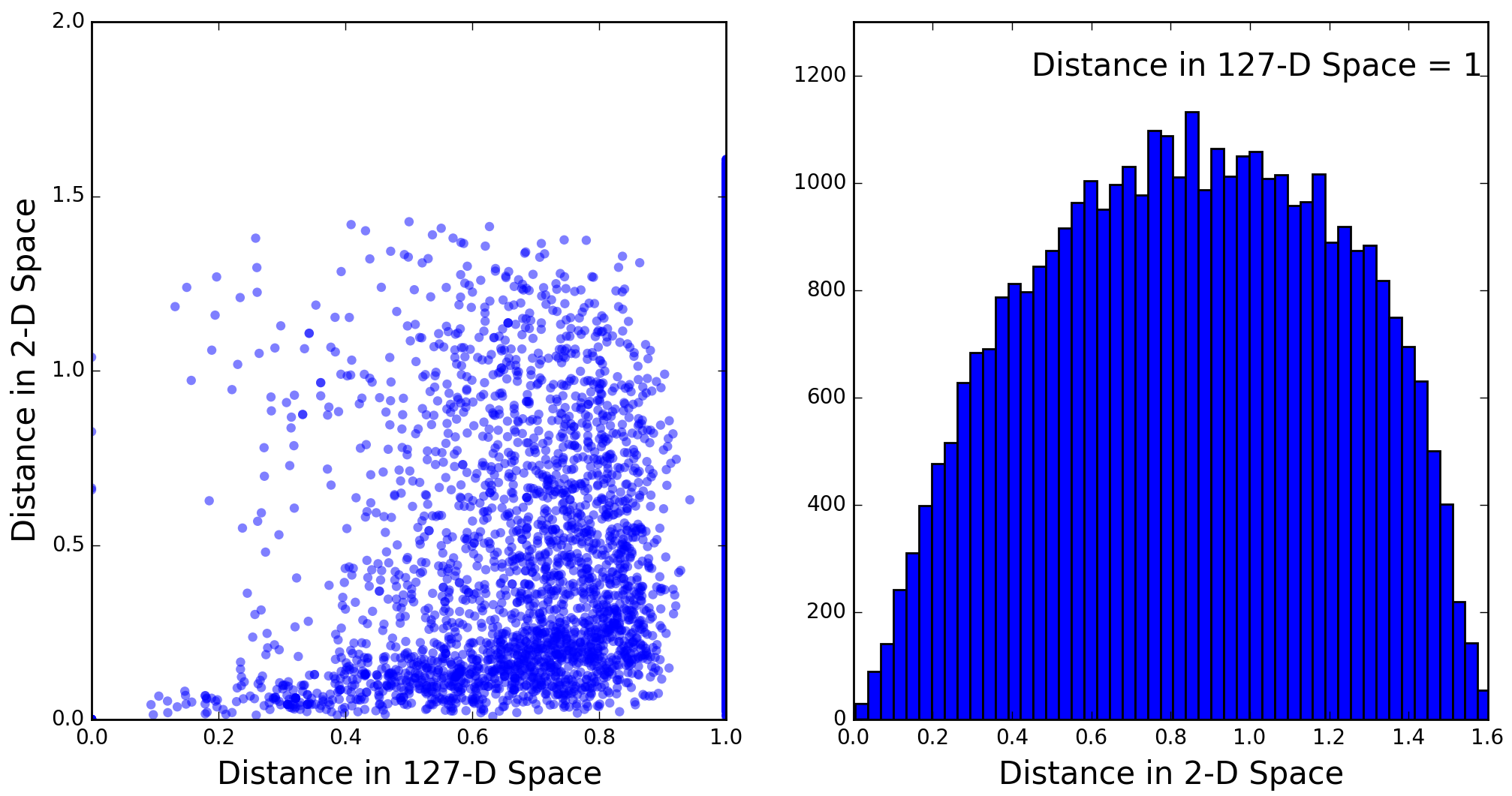
It is important to realize here that the 127-D distances are not true distances, but rather cosine similarities, which do not obey the triangle inequality and are bounded above by 1. This being said, the dark-blue band near the bottom in the plot on the left does indicate some correlation between distances in the two spaces, amid substantial noise. The “plume” of inter-tweet distances above the correlation band shows that, when we try to visualize clusters, we can expect some tweets belonging to a cluster to appear some distance away from that cluster. Conversely, the right-hand plot shows that a small fraction of tweets that are well separated in 127-D space may appear close in 2-D space. Hence the 2-D visualization of a cluster may be contaminated by unrelated tweets.
Clustering with K-Means
Like many clustering algorithms, K-means assumes that the number of clusters present in the data is known in advance. It starts with some (possibly random) locations for the cluster means, and associates each point in the data set to the closest cluster mean. The cluster means are then recomputed, and the process is repeated until the clusters are stable.
For the tweets dataset I certainly didn’t know the number of clusters in advance, but it turns out the algorithm is pretty good at identifying plausible clusters anyway. Assuming that the number of clusters is five, here is the result:
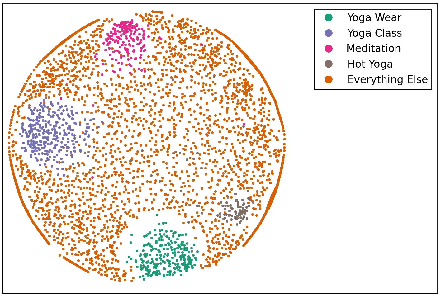
The K-means visualization with MDS works remarkably well for five clusters, in the sense that it identifies four of the most “obvious” clusters, and then throws everything else in the fifth cluster. The names I gave to the clusters in the legend of Figure 7 are attempts to summarize the most common n-grams found in the clustered tweets. For each cluster, the top n-grams as well as the number of tweets belonging to it are listed below:
Yoga Wear: ["pants", "yoga pants", "wear", "wear yoga pants", "wear yoga"], 436 tweets.
Yoga Class: ["class", "yoga class", "free", "going", "start", "join", "fitness", "today"], 346 tweets.
Meditation: ["meditate", "yoga meditate", "mudra", "yoga meditate mudra", "meditate mudra", "mind", "day", "going", "free", "relaxation"], 231 tweets.
Hot Yoga: ["hot", "hot yoga", "class", "follow", "tonight", "practice"], 136 tweets.
Everything Else: ["day", "get", "practice", "love", "poses", "time", "fitness", "today"], 3630 tweets.
As one increases the number of clusters, K-means keeps finding solutions (it always will), but the visualization becomes less compelling for higher-order clusters. Here is, for example, the result for 20 clusters:
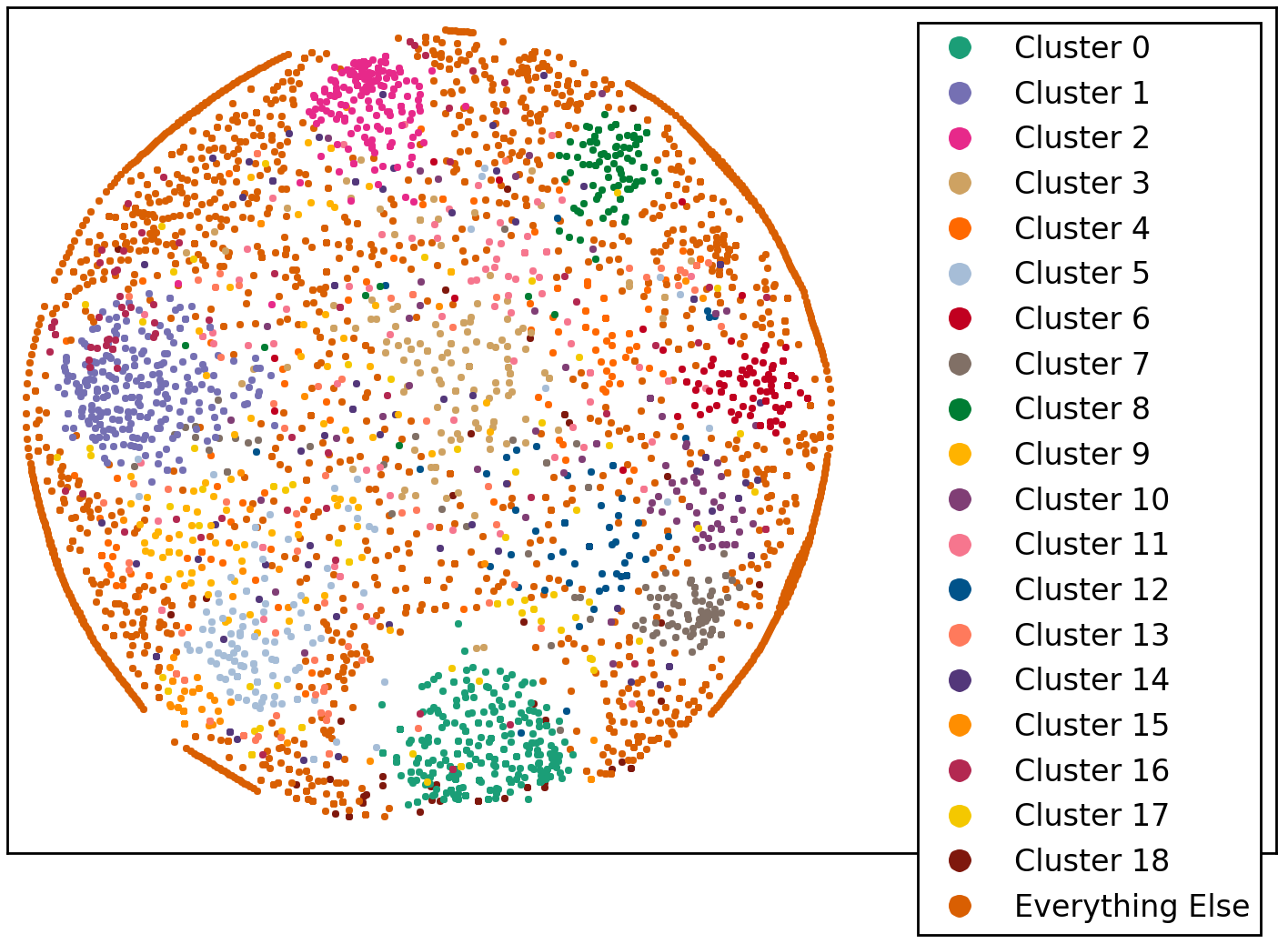
The five previously found clusters are still present, although with some minor contamination from other clusters. The cluster numbers in the legend of Figure 8 correspond to decreasing order of cluster population. The only exception is the very last cluster, labeled “Everything Else”, which is in fact the most populous one (2261 tweets) and appears to just fill the background in this visualization.
The top K-Means clusters by population do seem to reveal topics. Let’s now try a second approach, where we start from topics and then identify clusters.
Topic Modeling with Latent Dirichlet Allocation (LDA)
Latent Dirichlet Allocation models documents as probability distributions over topics, and topics as probability distributions over terms (n-grams). The pre-processing of tweets for LDA is similar to that for MDS and K-Means. The only difference is that we don’t use the “Idf” part of the Tf-Idf transformation, that is, terms within tweets are not weighted by their inverse document frequency.
Similar to K-Means, the LDA algorithm requires the user to specify the number of topics present in the corpus of documents, which is not a trivial issue. We’ll test the waters by setting the number of topics to five. To map topics into clusters of tweets, we associate each tweet with its most probable topic (recall that with LDA each tweet is a probability distribution over topics). Here is the result:
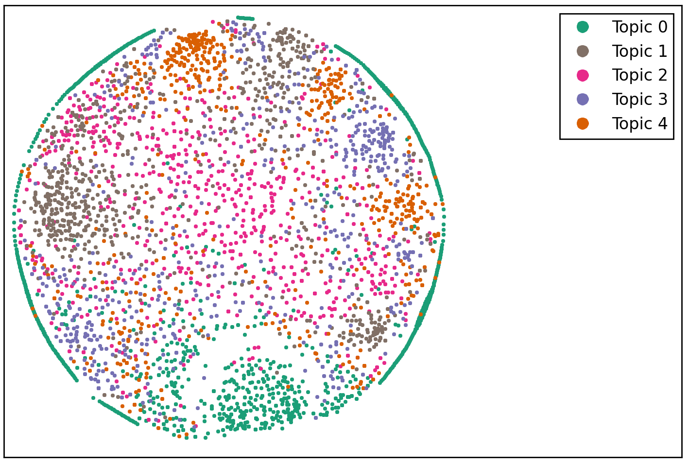
Compared with K-Means (Figure 7), LDA clusters have ‘blurry’ edges (see how Topic 0 leaks across the wide gap surrounding the K-Means “Yoga Wear” cluster). In addition, some LDA clusters are mixtures of K-Means clusters. For example, “Topic 1” is a mixture of the “Yoga Class” and “Hot Yoga” clusters of Figure 7, plus at least one other cluster.
One possible solution to the mixture and blurriness problems is to specify a larger number of topics for LDA to disentangle. Here is the result for 20 topics:
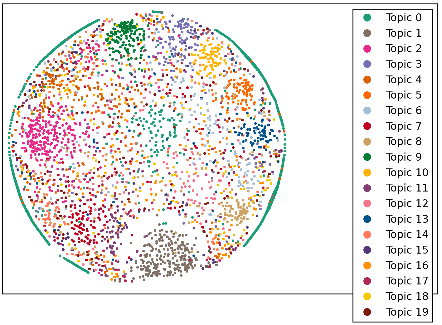
Cluster sharpness has improved considerably. For comparison with K-Means, here is LDA’s description of the four clusters common to Figures 10 and 7 (each feature below is “multiplied” by its LDA probability under the corresponding topic; probabilities should add up to 1 for each topic, but for brevity only the most significant features are listed):
Topic 1: 0.3745*"pants" + 0.3516*"yoga pants" + 0.0959*"wear" + 0.0449*"say" + 0.0418*"leggings", 434 tweets.
Topic 2: 0.3248*"class" + 0.2096*"yoga class" + 0.1148*"going" + 0.1013*"body" + 0.0889*"try", 408 tweets.
Topic 9: 0.3127*"meditate" + 0.1822*"yoga meditate" + 0.1070*"mudra" + 0.0988*"yoga meditate mudra" + 0.0988*"meditate mudra", 198 tweets.
Topic 8: 0.3185*"hot" + 0.2417*"look" + 0.2174*"hot yoga" + 0.1481*"studio", 201 tweets.
The top features per topic/cluster in LDA and K-Means overlap to a large degree, although not completely.
A second possible solution to the mixture and blurriness problems is to “seed” LDA topics. For example, we know from our K-Means analysis that there are topics associated with yoga wear, yoga classes, meditation, and hot yoga. By a priori reweighing appropriate model features we can get LDA to sharpen these topics. Here is the result for five topics, after reweighing the features "pant" and "wear" for Topic 1, "class" and "free" for Topic 2, "medit" and "mudra" for Topic 3, and "hot" for Topic 4, by a factor of 500 to 1 with respect to the other features:
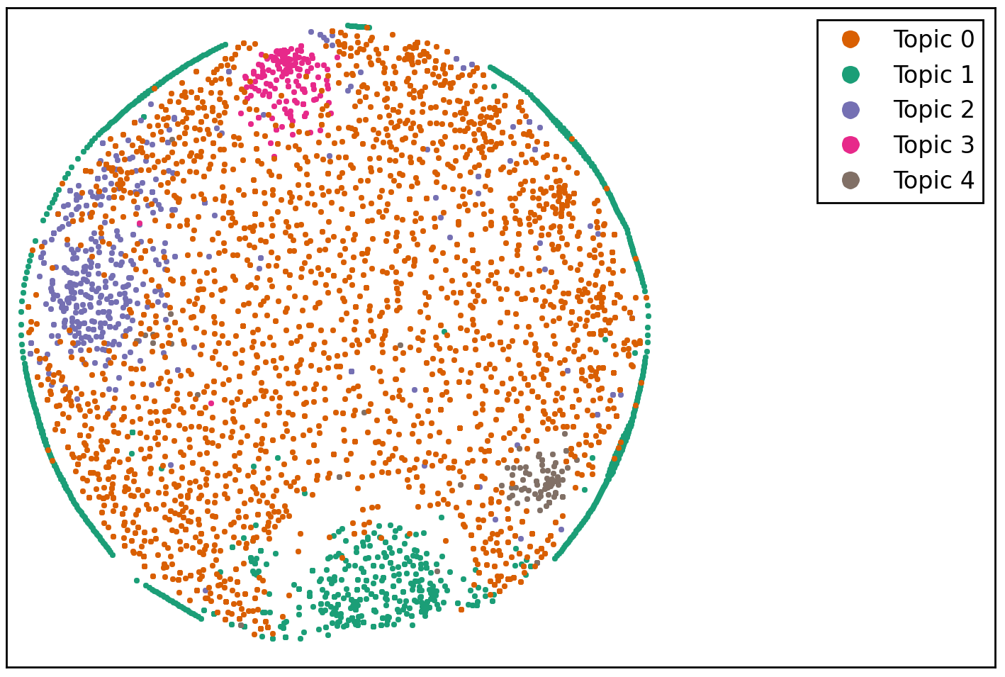
Cluster definition is much better here than on Figure 9, and is almost as good as the K-Means result of Figure 7.
Summary
In K-Means, the top n-grams attached to a cluster can be used to identify a topic associated with that cluster. In LDA, by grouping documents for which a given topic has the highest probability, one can associate a cluster with that topic. This mapping between topics and clusters can be used to compare K-Means and LDA.
Although K-Means requires specification of the number of clusters present in the data, it seems good at identifying well-defined clusters, even if the specified number of clusters is well below the actual number. This is not the case with LDA, which is very sensitive to the specified number of topics. On the other hand, LDA allows the user to seed a topic with a prior distribution over features (n-grams).
By making the input number of LDA topics sufficiently large, or by seeding topics, it is possible to obtain reasonable agreement between LDA and K-Means.
Technical Note
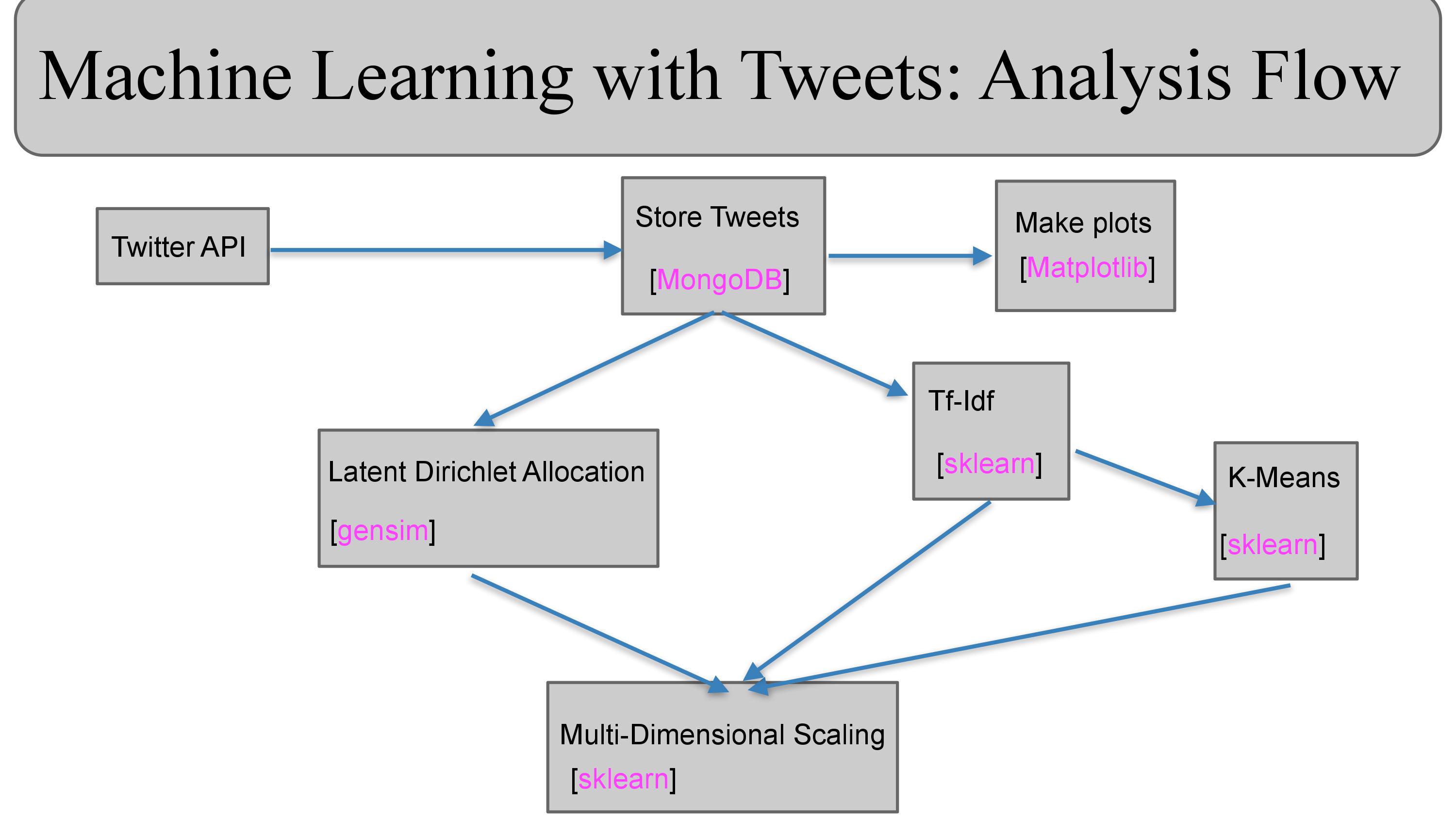
The analysis flow of this study is shown in Figure 12 below. The analysis code can be found in my GitHub repository.
