Metis Project Luther: Movies and Stars
April 24, 2015
[Revised 27 December 2023]
Suppose you had to advise a Hollywood investor about which movies are most likely to make a profit at the box office. How should you proceed? Before answering, consider what the Wikipedia entry on film finance says about one example of such advice: “[Ryan] Kavanaugh has attempted to use data from major studios like Sony and NBC/Universal to build a complex Monte Carlo system to determine movie failure rates prior to production. His projects and business models have failed miserably, causing a half-a-billion dollars in losses. The box office results of his movies have been mixed, as there is no set ratios, blends, mixtures, method or secret crystal ball that can project movie revenues, investor risk or rejection parameters.” Now what? This sounds pretty discouraging, but surely we can predict something about movie revenues, even if only probabilistically. For project Luther of the Metis data science bootcamp I investigated the question of how the “star value” of a cast can affect revenue.
Movie Data: Collection and Exploration
I obtained movie data for the years 2005-2014 by scraping the website of BoxOfficeMojo. Since I am looking at domestic movie casts and domestic revenue for this analysis, I filtered out foreign movies as well as documentaries from the sample. The distribution of the number of movies released over the years, before and after the filter, is shown in Figure 1 (left panel). The right panel shows the distribution of movie releases by month (summed over the years in the sample).

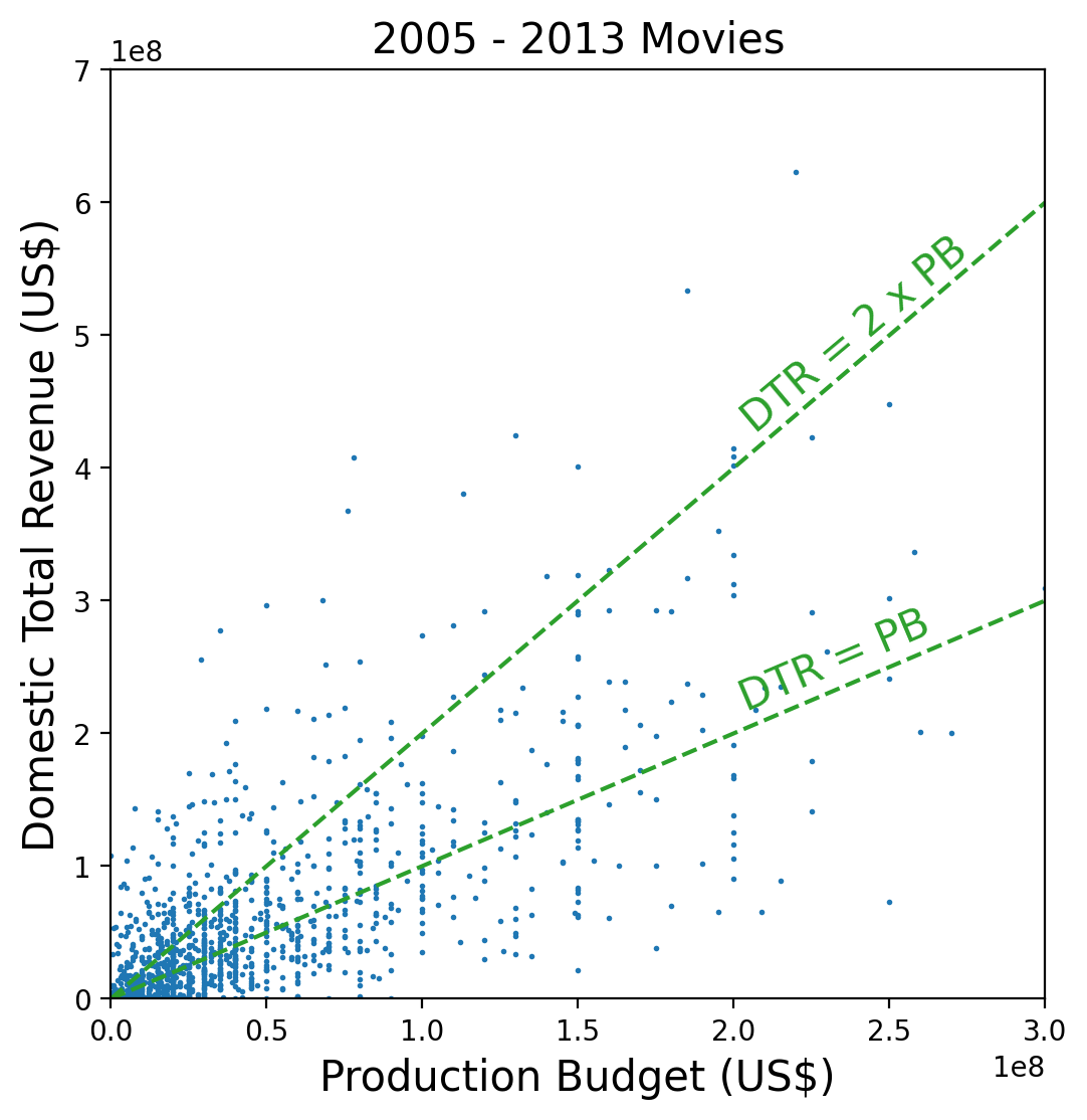
Figure 2: Domestic Total Revenue versus Production Budget for movies in the analysis sample. A linear scale is used on both axes. The dashed green lines are where domestic total revenue equals the production budget and twice the production budget.Each year sees the release of about 600 movies, with release dates peaking in early Spring and early Fall. Removing foreign movies and documentaries leaves about 400 movies per year. In total, the sample contains 6101 movies before filtering and 3832 movies after.
How well have movies done in the recent past? One way to answer this question is to plot total domestic revenue versus production budget. This is shown in Figure 2 for the years 2005-2013 (I left out 2014 for later testing purposes). Production budgets are typically rounded to the nearest tens of millions of dollars, which explains why some points in the figure are vertically aligned. Although this figure shows in detail the upper tail of the joint distribution of revenue and budget, it hides the lower tail. The latter is revealed by using a logarithmic scale on both axes, as done in the top-right panel of Figure 3.
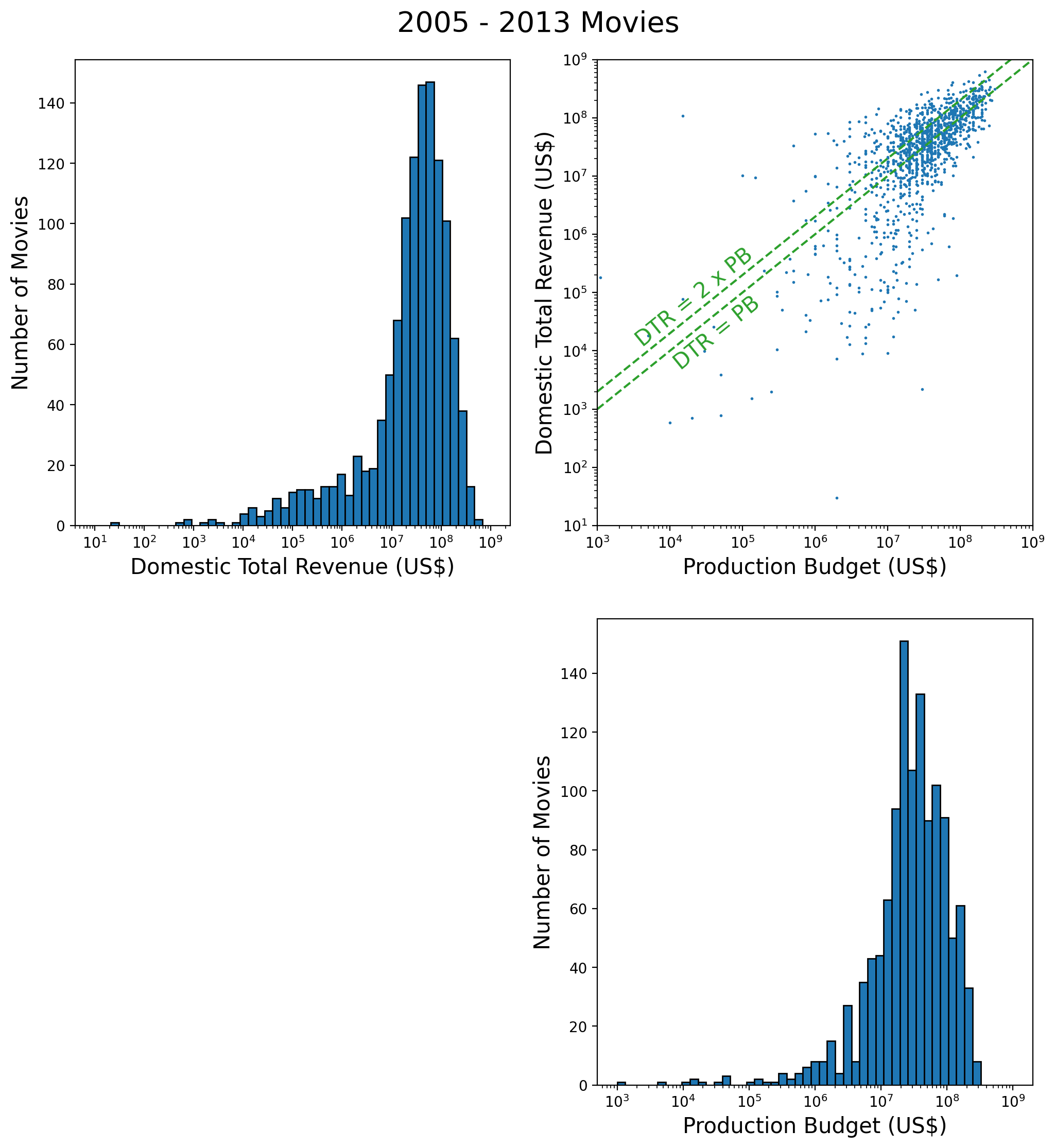
The top-right corner of the log-log version of the scatter plot shows how the revenue fluctuates around lines of near-zero profit, where domestic total revenue equals once or twice the production budgetBesides the production budget, profit is also affected by the promotional budget, which can be as substantial as the production budget (see for example this post by Charlie Jane Anders). As a rule of thumb, a movie needs to make twice its production budget to break even. . 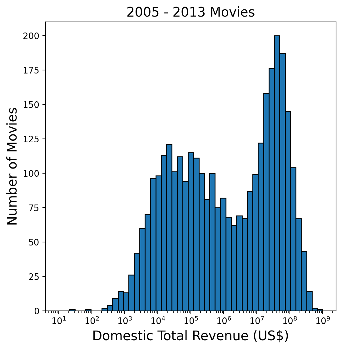
Figure 4: Distribution of Domestic Total Revenue for all movies, regardless of whether the Production Budget is known.There is a worrisome tail of movies with domestic total below about 2x10⁶: In this region there are remarkably few movies that make a profit. This is a good place to mention that this plot only contains 1206 movies, out of more than 3000 in the 2005-2013 sample, and that this is because the balance of movies don’t have a production budget listed on the BoxOfficeMojo website. If we plot a histogram of the domestic total revenue regardless of whether the production budget is known, we get Figure 4. This histogram contains 3313 movies and exhibits two peaks! Compared to the top-left panel of Figure 3, the new peak appears to the left of the main peak, precisely where the negative-profit movies show up on the Figure 3 scatter plot. One cannot help but speculate that all the movies for which no production budget is available were actually “flops”. Whereas this is pure speculation, it is hard to evade the conclusion that something systematic must be at work. Maybe the absence of a production budget correlates with some specific release years or months, or movie genres, or MPAA ratings? This is straightforward to check with the help of Figure 5 below.
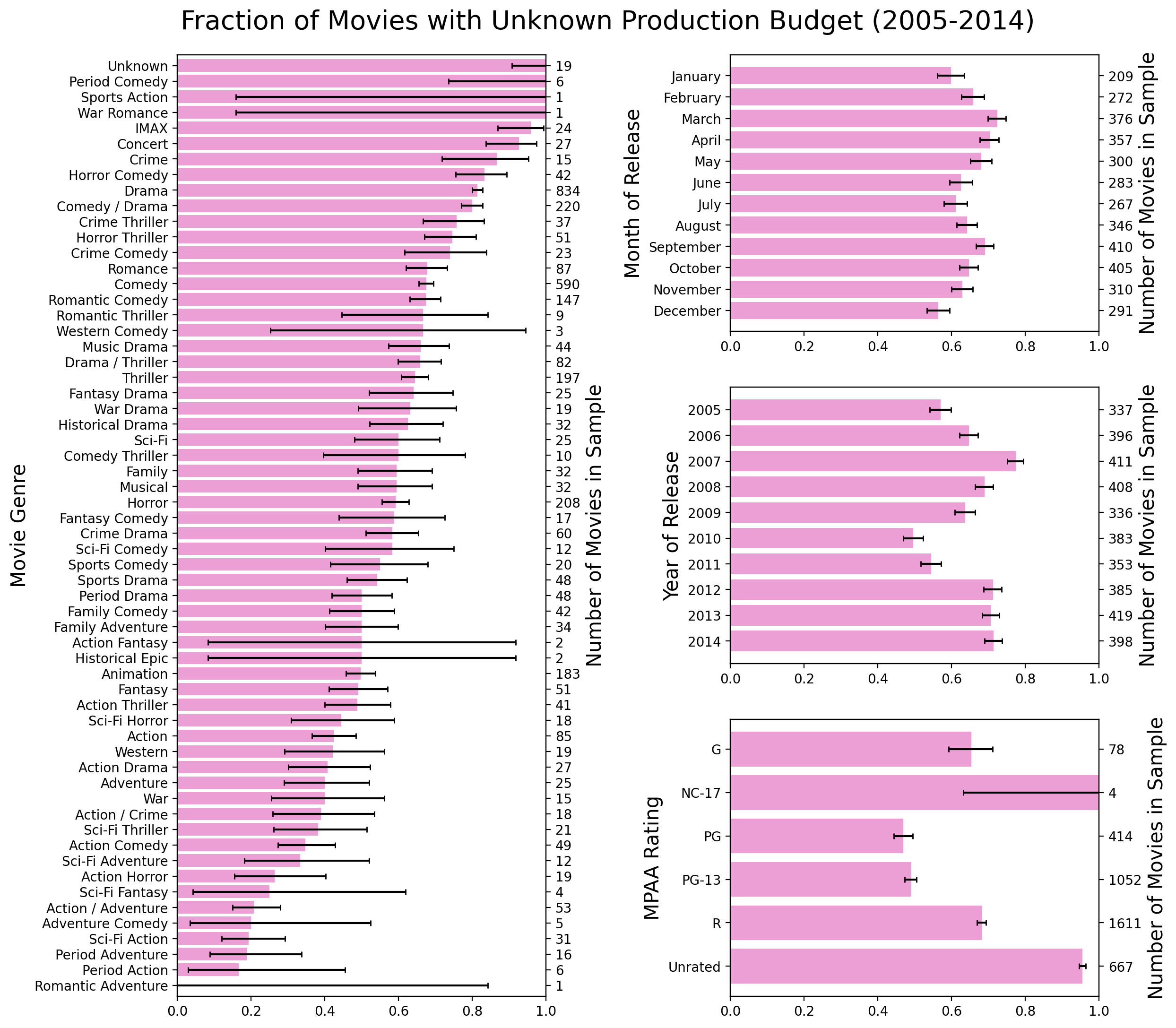
There is no obvious pattern: no single feature can account for the more than 2000 movies with unknown production budget in the sample. I won’t speculate any further on this issue, except to say that the source of the second peak in the distribution of domestic total revenue must be a random factor that is not explicitly provided in the BoxOfficeMojo data.
Cast Data: the Star Value of a Movie
Information about actors, actresses, and directors was obtained by scraping the Oscars website. Oscar nominations and wins were collected for the years 1949 to 2014. I defined the star value of a movie as follows:
Star value of a movie = Total number of Oscar wins and Oscar nominations by actors, actresses, and director of the movie in all previous years.
For example, Meryl Streep could contribute a maximum of 19 points to a movie’s star value (3 wins plus 16 nominations), Jack Nicholson 12 (3 plus 9), Paul Newman 9 (1 plus 8), Peter O’Toole 8 (0 plus 8), and Marlon Brando 8 (2 plus 6). The exact number of points contributed depends of course on the year of the movie’s release. The distribution of the star value over all movies in my sample is shown in the lower-right panel of Figure 6.
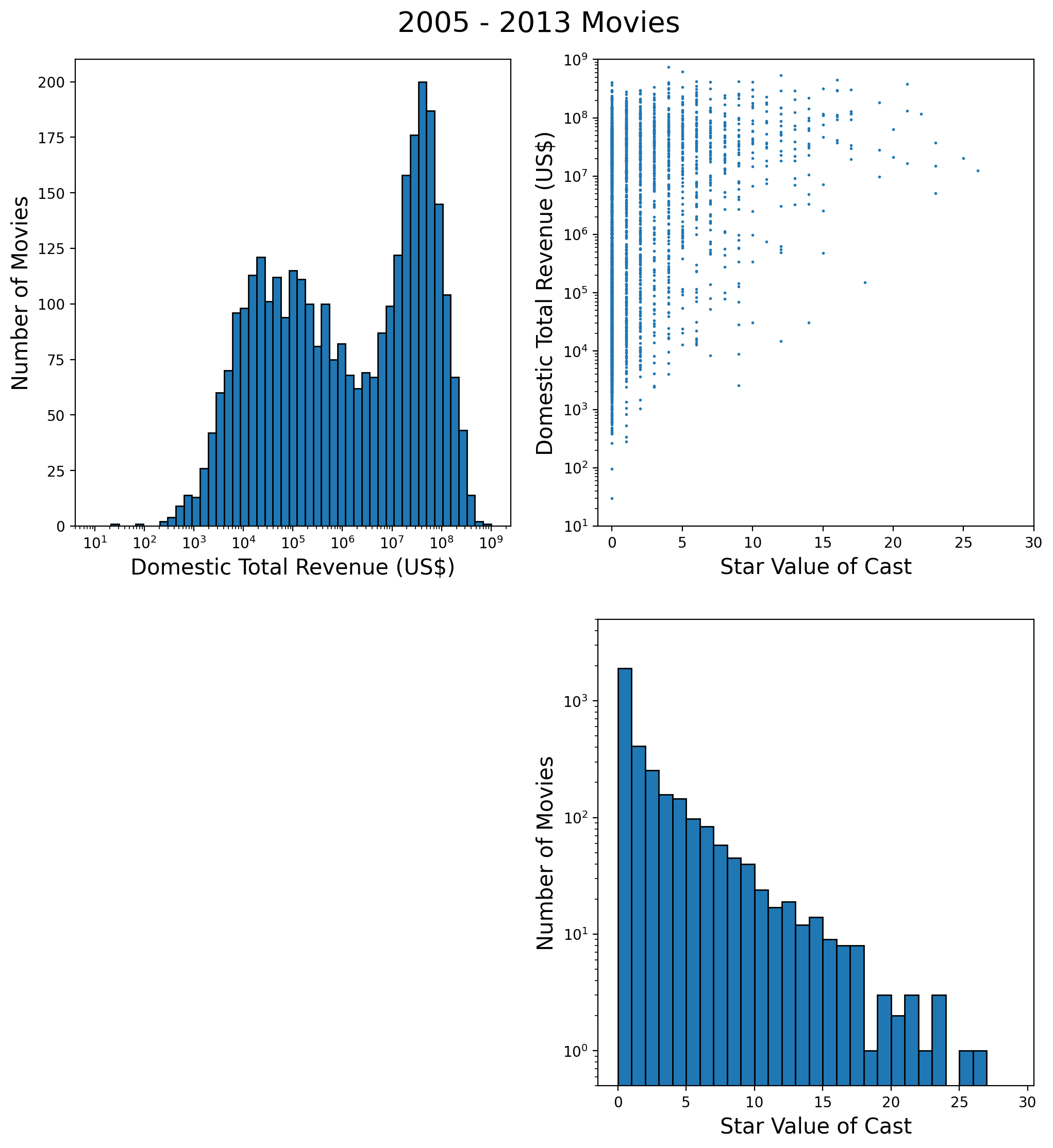
The upper-right panel shows a scatter plot of (log of) domestic revenue versus star value. It has a more-or-less triangular shape, such that movies with low revenue correspond to low star value, but not conversely.
Regression Analysis
From the scatter plot in Figure 6 it is clear that there cannot be a one-to-one relationship between the domestic total revenue of a movie and its star value. The relationship is affected by other random factors, which I have not explored. Therefore an Ordinary Linear Regression analysis cannot be applied. However this is a perfect case for the application of quantile regressionSee for example the Wikibooks page on quantile regression and references therein. . The question we seek to answer is: Given a star value, what is the lowest domestic revenue we can expect with (say) 90% confidence?
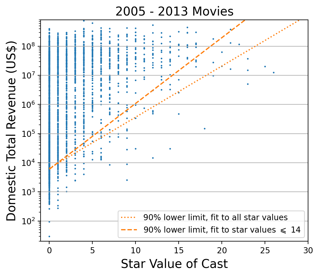
Figure 7: Domestic Total Revenue versus Star Value. Two quantile regression fits are shown: one that includes all data points (dotted line), and one that includes only data points with star value up to 14 (dashed line). Both fits estimate the 10th percentile of the revenue distribution as a function of star value, and therefore a 90% confidence-level lower bound on the revenue.I tried several models for the dependence of the log-revenue quantiles on the star value: linear, quadratic, cubic. Only a linear dependence gave satisfactory fits. However, the results depend on how many star values are included in the fit. There are few data points at high star values, making the fit somewhat uncertain in that region. I therefore tried two fits: one including all star values, and the second only including star values up to 14 (to guarantee at least ten data points per star value). The result is shown in Figure 7. If we count all the data points below the dotted line (the fit that includes all star values), we find 332, or 10.02% of the total (3313). If we count all the data points below the dashed line (the fit that includes all star values up to 14), we find 347, or 10.47% of the total. If we count all the data points below the dashed line and with star value up to 14, we find 328, which is 10.02% of the total number of points with star value no higher than 14 (3273).
Note that quantile regression does not require binning the data! It minimizes an objective function that only involves the coordinates of the individual data points. It is therefore interesting to check how the fit result compares with separate estimates of the log-revenue quantiles at each star value. This is shown in the left panel of Figure 8. The right panel of the same figure superimposes the fit results on 2014 movie data (which were not used in the fits).
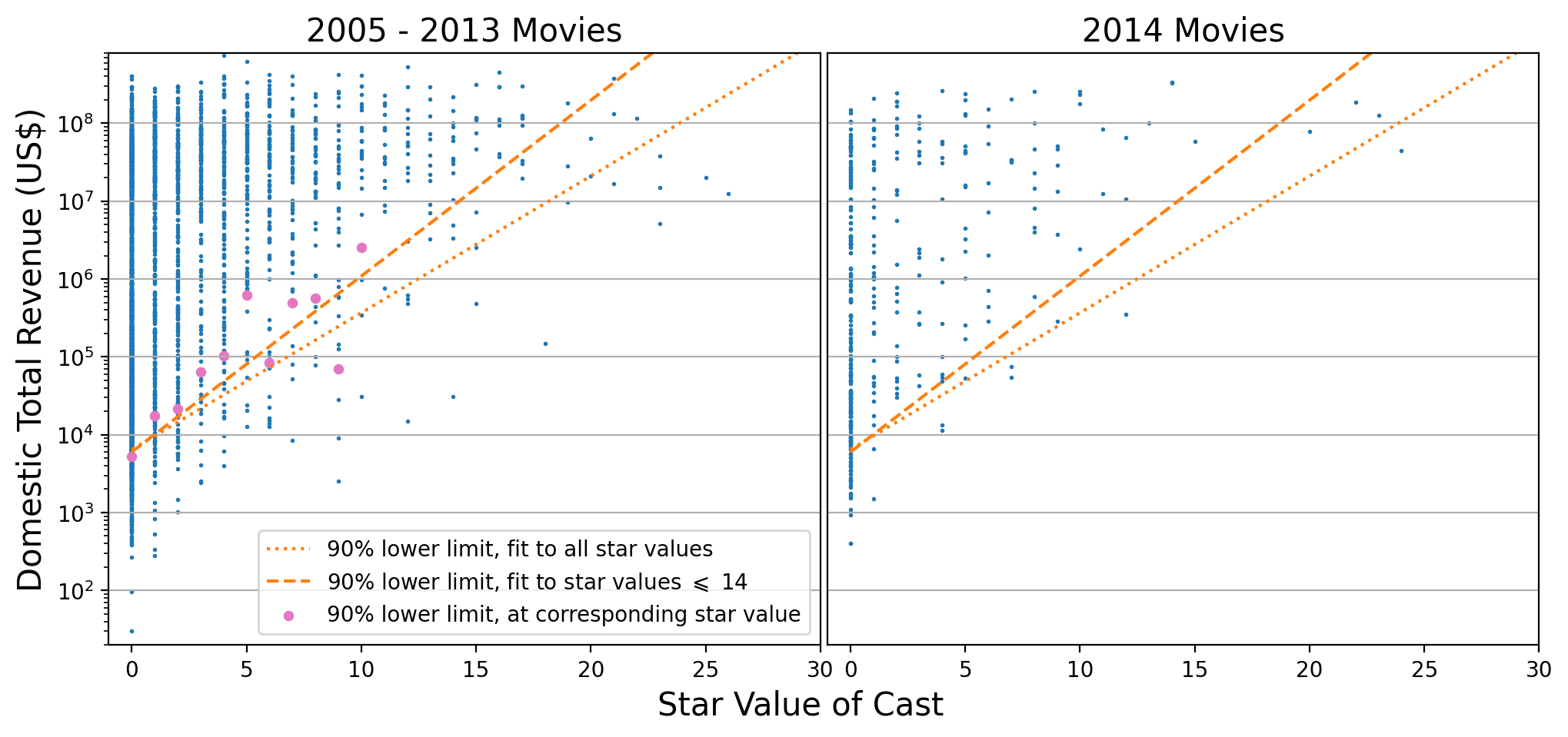
Both plots show reasonable agreement with expectations.
A significant advantage of quantile regression over ordinary regression is that the results remain valid under one-to-one transformations. In the present case I fitted log-revenue to star value. Hence, to obtain a relationship for revenue instead of log-revenue, it suffices to exponentiate the fit result. For the fit that includes only data points with star value up to 14 I found:
where is the tenth percentile of the distribution of total domestic revenues (in US dollars), and is the star value. For the fit that includes all data points I found:
Since this curve is mostly below the previous one (dotted versus dashed lines in Figure 7), it can be viewed as a conservative estimate of the 90% confidence-level lower bound on the expected revenue.
Refining the model
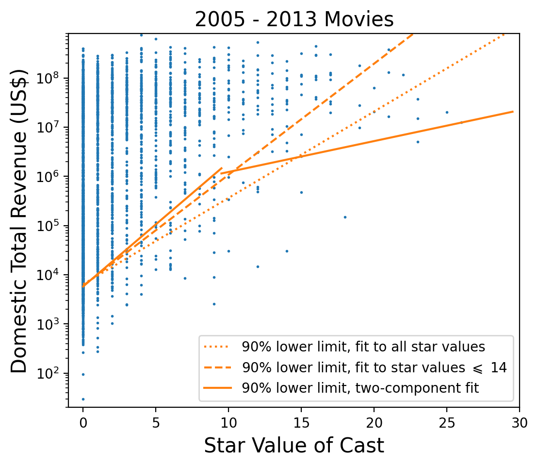
Figure 9: Logarithm of Domestic Total Revenue versus Star Value. A two-component quantile regression fit (solid lines) is shown on top of the data and compared with the previous fits (dotted and dashed lines).It is somewhat unsatisfactory that the linear model displayed in Figures 7 and 8 is so sensitive to the choice of endpoint for the fit. This can be understood as a saturation effect. The scatter plots suggest that the domestic total revenue has a constant upper bound of about one billion US dollars, regardless of the star value of the movie. Thus a linear model, which has revenue monotonically increasing with star value, cannot be correct. The revenue must turn over at high star value, i.e. saturate. Although this effect can be described with nonlinear models, I decided instead to try a two-component linear model. The idea is that the double-peak structure of the revenue distribution (Figure 4) should be taken into account in the fit. Looking at Figure 7, one could argue that the lower peak of the revenue distribution is only relevant for star values lower than or equal to 9. For higher star values the taller peak is the only one that matters. I therefore tried to fit these two regions separately to a linear model. The result is shown in Figure 9 and leads to the following parametrization of the 90% confidence-level lower bound:
The 90% confidence-level lower limit from the two-component model is slightly more “aggressive” than the other limits for star values less than 9, and is more conservative above 9.
Summary
We looked at domestic movie data from the years 2005-2014 and tried to correlate domestic revenue to the star value of a movie’s cast. The star value of a movie was defined as the total count of Oscar wins and nominations for all of the movie’s actors, actresses and director in years prior to the movie’s release. We found that the star value allows to set a probabilistic lower bound on the domestic revenue. Using quantile regression, we set 90% lower limits on revenue as a function of star value.
When deciding whether or not to invest in a movie’s production, one should of course look at expected profit rather than expected revenue. Therefore, combining the results of this study with information about the production budget should in principle prove useful to the decision maker.
Technical Note
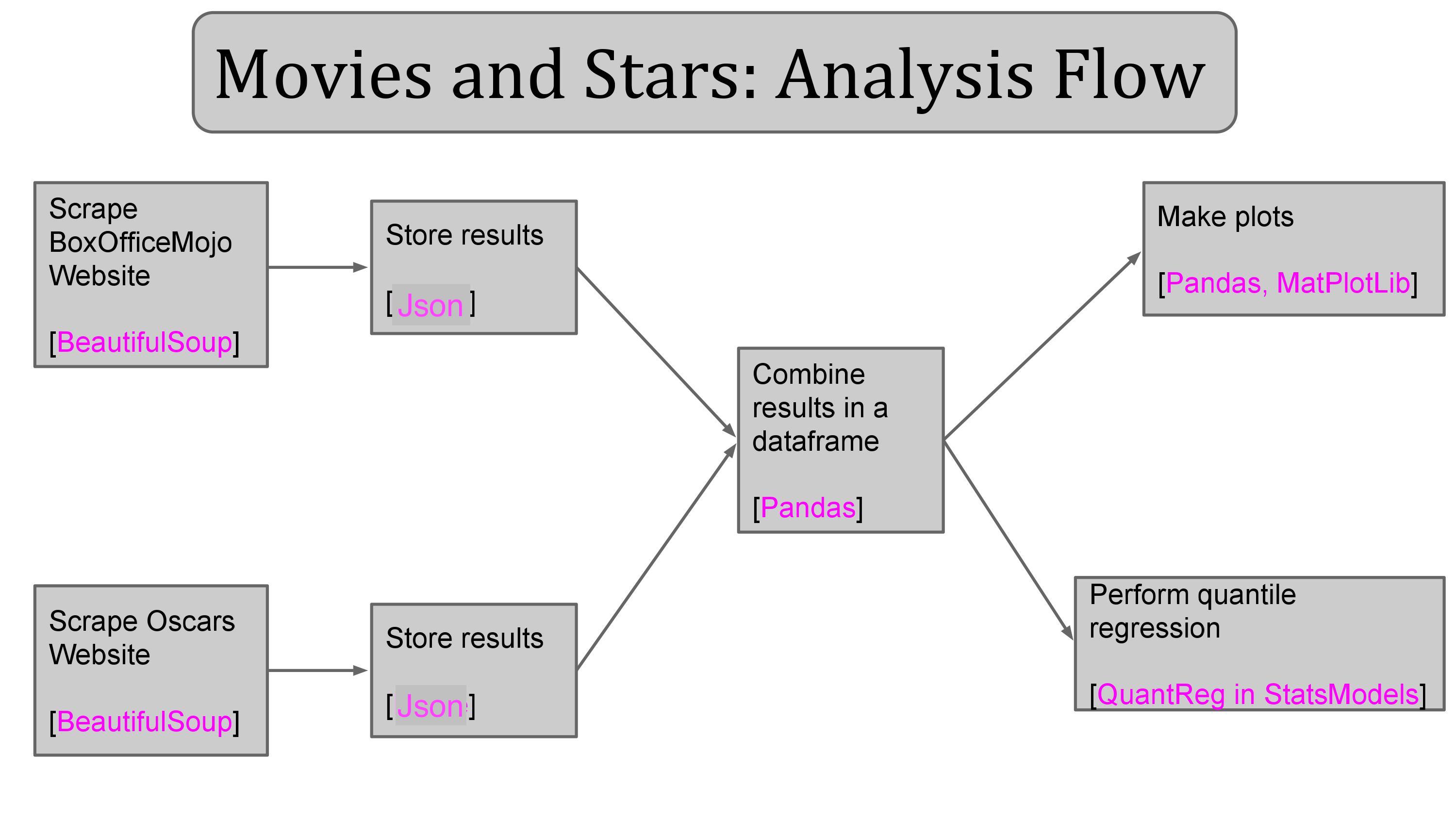
The diagram below shows the analysis flow of the present study together with the data science tools that I used. The analysis code can be found in my GitHub repository.
