Taking the Confusion out of the Confusion Matrix

July 26, 2016

[Last updated on 6 October 2024]

Contents
1. Introduction
2. Bayes’ theorem
2.1 Notation
2.2 The prior
2.3 The likelihood
2.4 The model evidence
2.5 The posterior
2.6 Classifier precision versus measurement precision
2.7 Summary
3. Joint probabilities
4. Likelihood ratios
5. When is a classifier useful?
6. Classifier scores
6.1 The receiver operating characteristic
6.2 The precision-recall curve
6.3 Classifier Scores and the Usefulness Conditions
7. Classifier operating points
8. Performance metric estimation
9. Trends and baselines
10. Effect of prevalence on classifier training and testing
11. Mathematical Appendix
11.1 Expectation values of sensitivity, specificity, and accuracy
11.2 Performance metrics versus threshold

1. Introduction

I always thought that the confusion matrix was rather aptly named, a reference not so much to the mixed performance of a classifier as to my own bewilderment at the number of measures of that performance. Recently however, I encountered a brief mention of the possibility of a Bayesian interpretation of performance measures, and this inspired me to explore the idea a little further. It’s not that Bayes’ theorem is needed to understand or apply the performance measures, but it acts as an organizing and connecting principle, which I find helpful. New concepts are easier to remember if they fit inside a good story.

Another advantage of taking the Bayesian route is that this forces us to view performance measures as probabilities, which are estimated from the confusion matrix. Elementary presentations tend to define performance metrics in terms of ratios of confusion matrix elements, thereby ignoring the effect of statistical fluctuations.

Bayes’ theorem is not the only way to generate performance metrics. One can also start from joint probabilities, likelihood ratios, or classifier scores. The next five sections describe these approaches one by one, and include a discussion of a minimal condition for a classifier to be useful. This is then followed by a section on estimating performance measures, one on the effect of changing the prevalence in the training and testing data sets of a classifier, and a technical appendix.

2. Bayes’ theorem

Let’s start from Bayes’ theorem in its general form:

$p(\lambda\mid X) \;=\; \frac{p(X\mid\lambda)\;\pi(\lambda)}{\int p(X\mid\lambda^{\prime})\;\pi(\lambda^{\prime})\;d\lambda^{\prime}}.$

Here $X$ represents the observed data and $\lambda$ a parameter of interest. On the left-hand side is the posterior probability density of $\lambda$ given $X$ . On the right-hand side, $p(X\mid\lambda)$ is the likelihood, or conditional probability density of $X$ given $\lambda$ , and $\pi(\lambda)$ is the prior probability density of $\lambda$ . The denominator is called marginal likelihood or model evidence. One way to think about Bayes’ theorem is that it uses the data $X$ to update the prior information $\pi(\lambda)$ about $\lambda$ , and returns the posterior $p(\lambda\mid X)$ .

For a binary classifier $\lambda$ is the true class to which instance $X$ belongs and can take only two values, say 0 and 1. The denominator in Bayes’ theorem then simplifies to:

$p(X) \;\equiv\; \int p(X\mid\lambda^{\prime})\;\pi(\lambda^{\prime})\;d\lambda^{\prime} \;=\; p(X\mid\lambda\!=\!0)\,\pi(\lambda\!=\!0)\;+\; p(X\mid\lambda\!=\!1)\,\pi(\lambda\!=\!1).$

We’ll take a look at each component of Bayes’ theorem in turn: the prior, the likelihood, the model evidence, and finally the posterior. Each of these maps to a classifier performance measure or a population characteristic. But first, a word about notation.

2.1 Notation

If our sole purpose is to describe the performance of a classifier in general terms, the data $X$ can be replaced by the class label $\ell$ or by the score $q$ assigned by the classifier (this score is not necessarily a probability and not necessarily between 0 and 1). Thus for example, $p(\lambda\!=\!1 \mid \ell\!=\!0)$ represents the posterior probability that the true class is 1 given a class label of 0, and $p(\lambda\!=\!1\mid q\!\ge\! q_{T})$ is the posterior probability that the true class is 1 given that the score $q$ is above a pre-specified threshold $q_{T}$ .

To simplify the notation we’ll write $\lambda_{0}$ to mean $\lambda=0$ , $\lambda_{1}$ to mean $\lambda=1$ , and similarly with $\ell_{0}$ and $\ell_{1}$ . Going one step further, where convenient we’ll write the prior as $\pi_{i}$ instead of $\pi(\lambda_{i})$ and the queue rate as $p_{i}$ instead of $p(\ell_{i})$ , where $i=0,1$ . With this notation the equation for the denominator of Bayes’ theorem becomes:

$p(X) \;=\; p(X\mid\lambda_{0})\,\pi_{0} \;+\; p(X\mid\lambda_{1})\,\pi_{1}.$

Finally, we’ll use the notation $A\;$ & $\;B$ to indicate the logical and of $A$ and $B$ , the notation $A \lor B$ for its logical or, and $A \mid B$ for the conditional $A$ given $B$ .

2.2 The prior

The first ingredient in the computation of the posterior is the prior $\pi(\lambda)$ . To fix ideas, let’s assume that $\lambda_{1}$ is the class of interest, generically labeled “positive”; it indicates “effect”, “signal”, “disease”, “fraud”, or “spam”, depending on the context. Then $\lambda_{0}$ indicates the lack of these things and is generically labeled “negative”. To fully specify the prior we just need $\pi_{1}$ , since $\pi_{0} = 1 - \pi_{1}$ . The prior probability $\pi_{1}$ of drawing a positive instance from the population is called the prevalence. It is a property of the population, not the classifier.

2.3 The likelihood

The next ingredient is the conditional probability $p(X\mid\lambda)$ . Working with the classifier label $\ell$ instead of $X$ leads to the following four combinations:

The true positive rate, also known as sensitivity or recall: $S_{e} \equiv p(\ell_{1}\mid \lambda_{1})$ ,
The true negative rate, also known as specificity: $S_{p}\equiv p(\ell_{0}\mid \lambda_{0})$ ,
The false-positive or Type-I-error rate: $\alpha\equiv p(\ell_{1}\mid\lambda_{0}) = 1 - S_{p}$ , and
The false-negative or Type-II-error rate: $\beta\equiv p(\ell_{0}\mid\lambda_{1}) = 1 - S_{e}$ .

For example, $p(\ell_{1}\mid \lambda_{0})$ is the conditional probability that the classifier assigns a label of 1 to an instance actually belonging to class 0. Note that the above four rates are independent of the prevalence and are therefore intrinsic properties of the classifier.

When viewed as a function of true class $\lambda$ , for fixed label $\ell$ , the conditional probability $p(\ell\mid\lambda)$ is known as the likelihood function. This functional aspect of $p(\ell\mid\lambda)$ is not really used here, but it is good to remember the terminology.

2.4 The model evidence

Finally, we need the normalization factor in Bayes’ theorem, the model evidence. For a binary classifier this has two components, corresponding to the two possible labels:

The positive labeling rate: $p_{1} = p(\ell_{1}\mid\lambda_{0})\,\pi_{0} + p(\ell_{1}\mid\lambda_{1})\,\pi_{1}$ , and
The negative labeling rate: $p_{0} = p(\ell_{0}\mid\lambda_{0})\,\pi_{0} + p(\ell_{0}\mid\lambda_{1})\,\pi_{1}$ .

The labeling rates are more commonly known as queue rates.

2.5 The posterior

Armed with the prior probability, the likelihood, and the model evidence, we can compute the posterior probability from Bayes’ theorem. There are four combinations of truth and label:

The positive predictive value, also known as precision: $\mathit{ppv}\equiv p(\lambda_{1}\mid\ell_{1}) = \frac{p(\ell_{1}\mid\lambda_{1})\, \pi_{1}}{p_{1}}$ ,
The negative predictive value: $\mathit{npv}\equiv p(\lambda_{0}\mid\ell_{0}) = \frac{p(\ell_{0}\mid\lambda_{0})\, \pi_{0}}{p_{0}}$ ,
The false discovery rate: $\mathit{fdr}\equiv p(\lambda_{0}\mid\ell_{1}) = 1 - \mathit{ppv}$ , and
The false omission rate: $\mathit{for}\equiv p(\lambda_{1}\mid\ell_{0}) = 1 - \mathit{npv}$ .

The precision, for example, quantifies the predictive value of a positive label by answering the question: If we see a positive label, what is the (posterior) probability that the true class is positive? (Note that the predictive values are not intrinsic properties of the classifier since they depend on the prevalence. Sometimes they are “standardized” by evaluating them at $\pi_{0} = \pi_{1} = 1/2$ .)

Figure 1 shows how the posterior probabilities $\mathit{ppv}$ , $\mathit{npv}$ , $\mathit{fdr}$ and $\mathit{for}$ are related to the likelihoods $S_{e}$ , $S_{p}$ , $\alpha$ and $\beta$ via Bayes’ theorem:

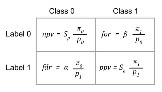
Figure 1: For each combination of class and label, Bayes' theorem connects the corresponding performance metrics of a classifier.

Note that if the operating point of the classifier is chosen in such a way that $p_{0} = \pi_{0}$ , we’ll have $\mathit{ppv} = S_{e}$ , $\mathit{npv} = S_{p}$ , and $\mathit{fdr}\times \mathit{for} = \alpha\times \beta$ .

2.6 Classifier precision versus measurement precision

Although we defined precision as a property of a classifier in a given population, there are reasons and ways to extend that definition to precision as a property of a measurement. Consider for example the Covid-19 pandemic. Tests for this disease are effectively classifiers, assigning negative and positive labels to members of the population. The positive predictive value of these tests depends on the prevalence $\pi_{1}$ , both directly and indirectly through the queue rate $p_{1}$ . We can make this dependence explicit:

$\mathit{ppv} \;=\; \frac{S_{e}}{S_{e} - \alpha + \alpha\left/\pi_{1}\right.},$

showing that $\mathit{ppv}$ will decrease if $\pi_{1}$ does. Suppose now that I take the test, and the result is positive. What are the chances that I actually have the disease? One answer would be the positive predictive value. However that number describes the test performance in the population and does not reflect the particular circumstances of my life. If I have no symptoms, and remained at home in isolation for the past two weeks, it seems unlikely that I would actually have the disease. This is where it is useful to remember the Bayesian construction of $\mathit{ppv}$ as the posterior probability obtained by updating the prior $\pi_{1}$ with the data from a test result. If we are talking about my particular test result, this prior should fold in more information than just the population prevalence. It should take into account the precautions I took as an individual, which could reduce $\pi_{1}$ significantly, and therefore also $\mathit{ppv}$ . The question of how exactly one should estimate prior probabilities is beyond the scope of this blog post, but the distinction between classifier precision and measurement precision is an important one to keep in mind.

2.7 Summary

This section introduced twelve quantities:

$\pi_{0},\; \pi_{1},\; S_{e},\; S_{p},\; \alpha,\; \beta,\; p_{0},\; p_{1},\; \mathit{ppv},\; \mathit{npv},\; \mathit{fdr},\; \mathit{for}.$

Only three of these are independent, say $\pi_{1}$ , $\alpha$ and $\beta$ , or $\pi_{1}$ , $S_{e}$ and $S_{p}$ . To see this, note that by virtue of their definition the first six quantities satisfy three conditions:

$\pi_{0} + \pi_{1} = 1,\quad S_{e} + \beta = 1, \quad S_{p} + \alpha = 1,$

and the last six can be expressed in terms of the first six: for $p_{0}$ and $p_{1}$ we have:

$p_{0} = S_{p} \pi_{0} + \beta \pi_{1}, \quad p_{1} = \alpha \pi_{0} + S_{e} \pi_{1},$

and Bayes’ theorem takes care of the remaining four (Figure 1).

The final number of independent quantities matches the number of degrees of freedom of a two-by-two contingency table such as the confusion matrix, which is used to estimate all twelve quantities (see below). It also tells us that we only need two numbers to fully characterize a binary classifier (since $\pi_{1}$ is not a classifier property). As trivial examples, consider the majority and minority classifiers. Assume that class 0 is more prevalent than class 1. Then the majority classifier assigns the label 0 to every instance and has $\alpha=0$ and $\beta=1$ . The minority classifier assigns the label 1 to every instance and has $\alpha=1$ and $\beta=0$ . These classifiers are of course not very useful. As we will show below, for a classifier to be useful, it must satisfy $\alpha + \beta \lt 1$ .

3. Joint probabilities

In some sense the most useful measures of classifier performance are conditional probabilities. By conditioning on something, we do not need to know whether or how that something is realized in order to make a valid statement. For example, by conditioning on true class, we ignore the prevalence when evaluating sensitivity and specificity. Similarly, conditioning on class label allows us to evaluate the predictive values while ignoring the actual queue rate.

In contrast, joint probabilities typically require more specification about the classifier and/or the population of interest, and are therefore less general than conditional probabilities. Nevertheless, by combining joint probabilities one can still obtain useful metrics. Start for example with the joint probability for class label and true class to be positive:

$p(\ell_{1} \;\&\; \lambda_{1}).$

Adding the joint probability for class label to be positive and true class to be negative yields the positive queue rate introduced earlier:

$p(\ell_{1} \;\&\; \lambda_{1}) \;+\; p(\ell_{1} \;\&\; \lambda_{0}) \;=\; p(\ell_{1}\mid\lambda_{1})\,\pi_{1} \;+\; p(\ell_{1}\mid\lambda_{0})\,\pi_{0} \;=\; p_{1}.$

If, instead, we add the joint probability for class label and true class to be negative, we obtain the so-called accuracy:

$p(\ell_{1} \;\&\; \lambda_{1}) \;+\; p(\ell_{0} \;\&\; \lambda_{0}) \;=\; p[(\ell_{1} \;\&\; \lambda_{1}) \;\lor\; (\ell_{0} \;\&\; \lambda_{0})] \;=\; p(\ell \!=\! \lambda) \;=\; {\rm A}.$

In terms of quantities introduced previously this is:

$\begin{align} {\rm A} \;=\; p(\ell_{1} \;\&\; \lambda_{1}) \;+\; p(\ell_{0} \;\&\; \lambda_{0}) &\;=\; p(\ell_{1}\mid\lambda_{1})\,\pi_{1} \;+\; p(\ell_{0}\mid\lambda_{0})\,\pi_{0} \;=\; S_{e}\,\pi_{1} \;+\; S_{p}\,\pi_{0}\\[1mm] &\;=\; p(\lambda_{1}\mid\ell_{1})\,p_{1} \;+\; p(\lambda_{0}\mid\ell_{0})\,p_{0} \;=\; \mathit{ppv}\,p_{1} \;+\; \mathit{npv}\,p_{0}. \end{align}$

Note the dependence on prevalence or queue rate. An equivalent measure is the misclassification rate, defined as one minus the accuracy. A benchmark that is sometimes used is the null error rate, defined as the misclassification rate of a classifier that always predicts the majority class. It is equal to $\min\{\pi_{0}, \pi_{1}\}$ . The complement of the null error rate is the null accuracy, which is equal to $\max\{\pi_{0}, \pi_{1}\}$ .

Note that null accuracy and null error rate are not necessarily good, or even reasonable benchmarks. In a highly imbalanced dataset for example, the classifier that always predicts the majority class will appear to have excellent performance even though it does not use any relevant information in the data.

4. Likelihood ratios

In some fields it is customary to work with ratios of probabilities rather than with the probabilities themselves. Thus one defines:

The positive likelihood ratio: ${\rm lr+} \equiv \frac{p(\ell_{1}\mid\lambda_{1})}{p(\ell_{1}\mid\lambda_{0})} = \frac{S_{e}}{1-S_{p}}$ , which represents the odds of the true class being positive if the label is positive (in medical statistics for example, this would be the odds of disease if the test result is positive).
The negative likelihood ratio: ${\rm lr-} \equiv \frac{p(\ell_{0}\mid\lambda_{1})}{p(\ell_{0}\mid\lambda_{0})} = \frac{1-S_{e}}{S_{p}}$ , which represents the odds of the true class being positive if the label is negative (in medical statistics, the odds of disease if the test result is negative).

Finally, it is instructive to take the ratio of these two likelihood ratios. This yields

The diagnostic odds ratio: $\mathit{dor} \equiv \frac{\rm lr+}{\rm lr-} = \frac{S_{e}}{1-S_{p}}\frac{S_{p}}{1-S_{e}}$ .

If $\mathit{dor} \gt 1$ , the classifier is deemed useful, since this means that, in our medical example, the odds of disease are higher when the test result is positive than when it is negative. If $\mathit{dor}=1$ the classifier is useless, but if $\mathit{dor}\lt 1$ the classifier is worse than useless, it is misleading. In this case one would be better off swapping the labels on the classifier output.

Note that the ratios ${\rm lr+}$ , ${\rm lr-}$ , and $\mathit{dor}$ are all independent of prevalence.

5. When is a classifier useful?

The usefulness condition $\fbox{$\mathit{dor} \gt 1$}$ is mathematically equivalent to any of the following conditions:

$\fbox{$S_{e}\gt 1 - S_{p}$}$ The sensitivity must be larger than one minus the specificity. Equivalently, the probability of detecting a positive-class instance must be larger than the probability of mislabeling a negative-class instance. Reformulating in terms of Type-I and II error rates this condition becomes $\fbox{$\beta \lt 1 - \alpha$}$ .
$\fbox{$S_{e} \gt p_{1}$}$ The probability of encountering a positively labeled instance must be larger within the subset of positive-class instances than within the entire population. Similarly: $\fbox{$S_{p} \gt p_{0}$}$ , $\fbox{$\alpha \lt p_{1}$}$ , and $\fbox{$\beta \lt p_{0}$}$ .
$\fbox{$\mathit{ppv} \gt \pi_{1}$}$ The precision must be larger than the prevalence. In other words, the probability for an instance to belong to the positive class must be larger within the subset of instances with a positive label than within the entire population. If this is not the case, the classifier adds no useful information. Similarly: $\fbox{$\mathit{npv} \gt \pi_{0}$}$ , $\fbox{$\mathit{fdr} \lt \pi_{0}$}$ , and $\fbox{$\mathit{for} \lt \pi_{1}$}$ .

The classifier usefulness condition also puts a bound on the accuracy (but is not equivalent to it):

${\rm A} \;=\; S_{e}\,\pi_{1} \;+\; S_{p}\,\pi_{0} \;>\; p_{1}\,\pi_{1} \;+\; p_{0}\,\pi_{0}.$

Since $p_{0} + p_{1} = 1$ , the right-hand side of the above inequality is bounded between $\min(\pi_{0}, \pi_{1})$ and $\max(\pi_{0}, \pi_{1})$ . The upper bound is actually the accuracy of the majority classifier, which assigns the majority label to every instance. Note that the majority classifier itself is not a useful classifier, since its accuracy is equal to its corresponding bound, not strictly higher than it. In addition, it is entirely possible for a useful classifier to have an accuracy below that of the useless majority classifier. To illustrate this last point, consider the minority classifier, which assigns the minority label to every instance. This is a useless classifier, with accuracy $\pi_{1}$ if we assume that $\pi_{1} \lt \pi_{0}$ . To improve it, let’s flip the label of one arbitrarily chosen majority instance. The accuracy of this new classifier is $\pi_{1} + 1/N$ , with $N$ the size of the total population (assumed finite in this example). This is larger than the accuracy bound, $p_{1}\pi_{1} + p_{0}\pi_{0} = \pi_{1} + 1/N - 2\pi_{1}/N$ . Hence the new classifier is useful, even though for $N$ large enough its accuracy will be lower than that of the majority classifier. Of course for other metrics the new classifier performs better than the majority one, for example sensitivity and the predictive values.

6. Classifier scores

As mentioned earlier, classifiers usually produce a score $q$ to quantify the likelihood that an instance belongs to the positive class. The performance metrics introduced so far can be defined in terms of this score, but they only need it in a binary way, through the class label $\ell$ : $\ell=1$ if $q\ge q_{T}$ , otherwise $\ell=0$ , for some predefined threshold $q_{T}$ . The next two performance metrics we discuss use score values without reference to $q_{T}$ .

6.1 The Receiver Operating Characteristic (ROC)

The Receiver Operating Characteristic, or ROC, is defined as the curve of true positive rate versus false positive rate (or sensitivity versus one-minus-specificity). An example is shown in the figure below:

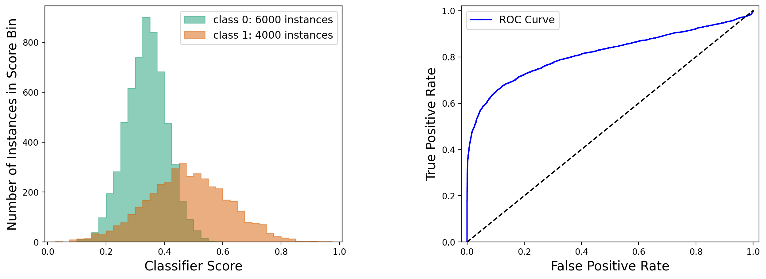
Figure 2. Left: arbitrary classifier score distributions used for illustration. Right: corresponding ROC curve, obtained by varying the classifier threshold over the range of scores. In this example the area under the ROC is about 0.815.

Note how the main diagonal line $S_{e} = 1 - S_{p}$ serves as baseline in the ROC plot, in accordance with the classifier usefulness condition $S_{e} \gt 1 - S_{p}$ discussed in section 5.

The area under the ROC curve, or AUROC, is a performance metric that’s independent of prevalence and does not require a choice of threshold $q_{T}$ on the classifier score $q$ . In other words, it does not depend on the chosen operating point of the classifier. It can be shown that the AUROC is equal to the probability for a random positive instance to be scored higher than a random negative instance.

An immediate interpretation of the AUROC is that it quantifies how well the score distributions for positive and negative instances are separated. If the score distribution for positives is to the right of that for negatives, and there is no overlap, the AUROC equals 1. If the positives are all to the left of the negatives, the AUROC equals 0, and if the two distributions overlap each other exactly, the AUROC equals 0.5.

The AUROC is related to expectation values of sensitivity, specificity, and accuracy (see appendix 11.1 for a proof):

$\begin{align} \mathbb{E}\left[S_{e}\right] \;&=\; \pi_{0}\, \textrm{AUROC} \;+\; \frac{\pi_{1}}{2},\\ \mathbb{E}\left[S_{p}\right] \;&=\; \pi_{1}\, \textrm{AUROC} \;+\; \frac{\pi_{0}}{2},\\ \mathbb{E}\left[A\right] \;&=\; 2\,\pi_{0}\,\pi_{1}\,\textrm{AUROC} \,+\, \frac{\pi_{0}^{2} + \pi_{1}^{2}}{2}, \end{align}$

where the expectation values are over an ensemble of identical classifiers with operating points that are randomly drawn from the distribution of scores of the population of interest. These equations demonstrate how the AUROC aggregates classifier performance information in a way that’s independent of prevalence and operating point (see also this answer by Peter Flach on Quora).

As we saw earlier, only three quantities are needed to determined all the performance characteristics of a classifier. We can take these to be the prevalence $\pi_{1}$ , the sensitivity $S_{e}$ , and the specificity $S_{p}$ . Thus, for a given value of the prevalence, each point on the ROC is associated with a unique value of, say, the precision. We can illustrate this by superimposing a colored map of precision on top of the ROC:

Figure 3. Left: ROC curve for a classifier in a balanced dataset, with a color map of the precision superimposed. Right: ROC curve and precision for the same classifier in the same dataset but with a lower prevalence.

The figure shows how the ROC curve is independent of prevalence, whereas the precision is not.

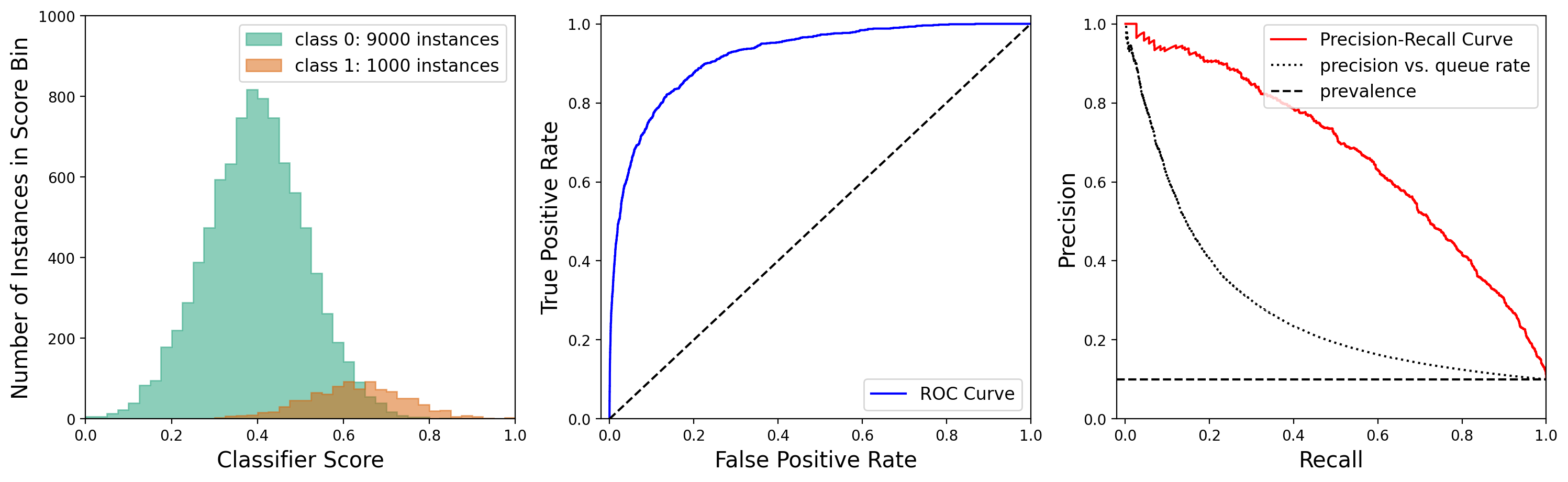
6.2 The Precision-Recall Curve (PRC)

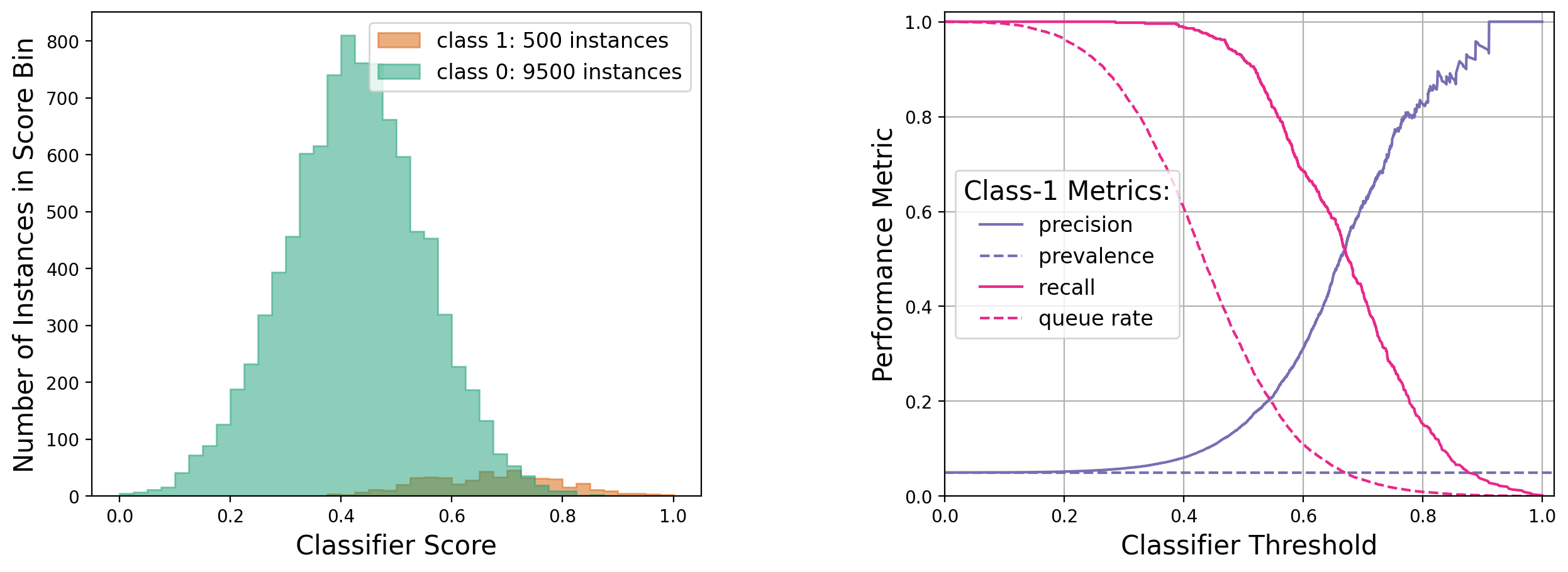
In cases where there is severe class imbalance in the data, the ROC may give too optimistic a view of classifier performance, because the true and false positive rates are both independent of prevalence, whereas precision deteriorates at low prevalence. It may therefore be preferable to plot a precision versus recall curve (or PRC). In the two illustrations below, the class distributions are the same, and only the class-1 prevalence is different. It can be seen that the ROC is independent of prevalence and looks quite good. On the other hand, the precision versus recall curve shows that the classifier performance leaves quite a bit to be desired in the case of imbalanced data. One can also calculate the area under the precision versus recall curve (or AUPRC) to summarize this effect.

Figure 4. Balanced dataset: classifier score distributions (a), metrics vs. threshold (b), ROC (c), and PRC (d). The areas under the ROC and the PRC are both about 0.92.

Figure 5. Imbalanced dataset: classifier score distributions (a), metrics vs. threshold (b), ROC (c), and PRC(d). In this case the area under the ROC is still about 0.92 whereas that under the PRC is now 0.65.

6.3 Classifier Scores and the Usefulness Conditions

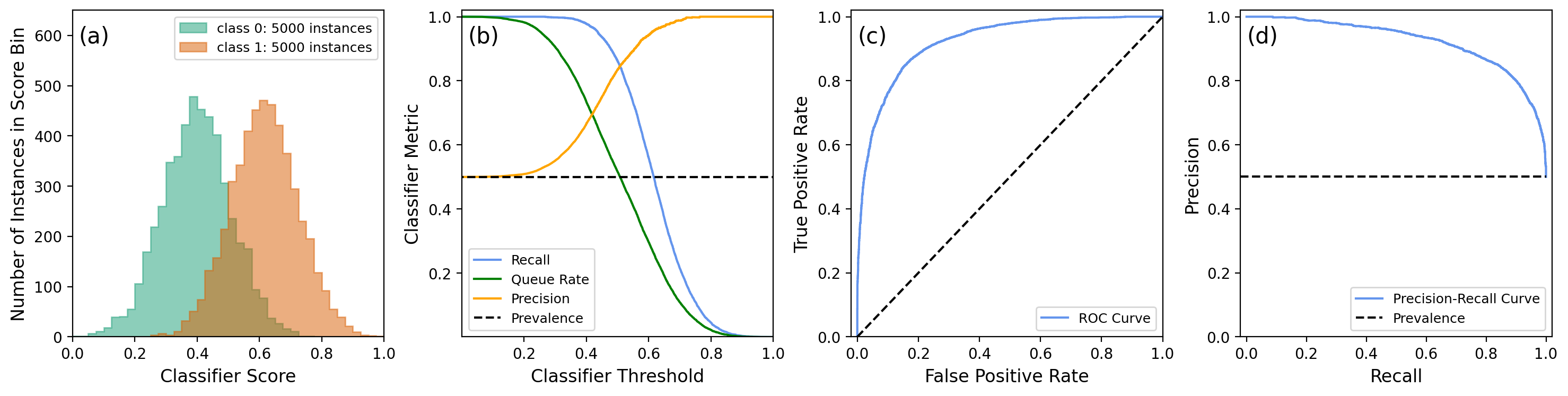
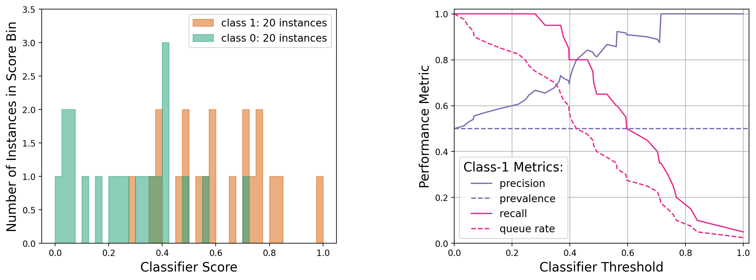
The classifier usefulness conditions discussed in section 5 apply to every threshold setting of a classifier with scores. This can lead to non-trivial situations, for example when a few negative-class instances are scored higher than the highest-score positive-class instance. To illustrate this, we consider an exaggerated example in the figures below.

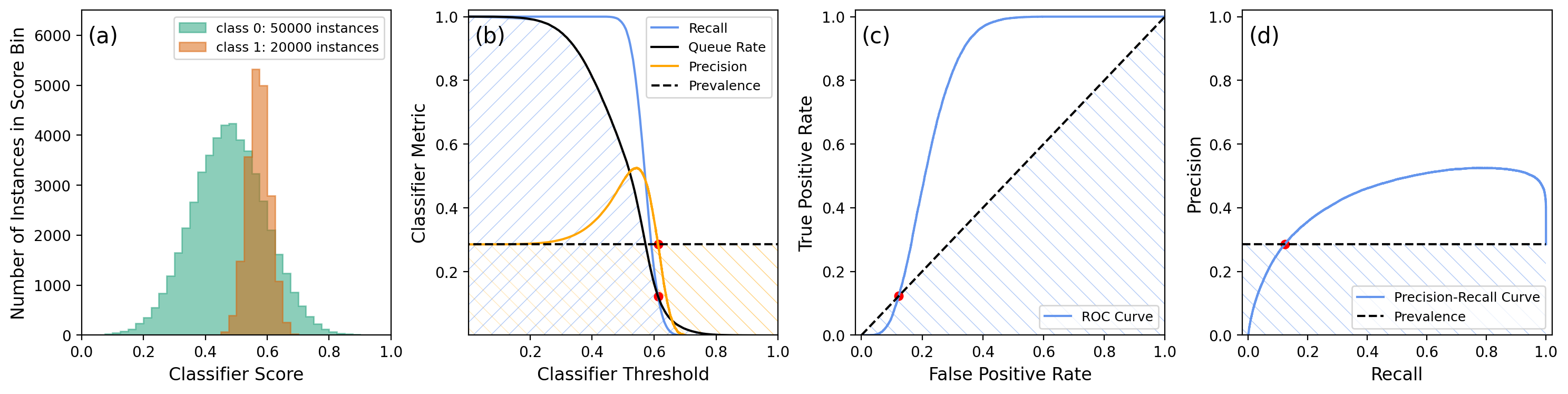
Figure 6. Classifier score distributions in an imbalanced dataset where some class-0 instances extend beyond the class-1 distribution (a), metrics vs. threshold (b), ROC (c), and PRC (d). The area under the ROC is about 0.78, and the area under the PRC is 0.43.

Note how the classifier usefulness conditions are violated. In panel (b), the precision dips below the prevalence, and the recall below the queue rate, at a threshold of about 0.61, where the recall equals 0.123. In panel (c) true positive rates lower than 0.123 are below the corresponding false positive rates, and in panel (d) the precision is lower than the prevalence when the recall is lower than 0.123. In the last three panels, the classifier is useless when its threshold is in a region where one of the colored curves has crossed into a hatched area of the same color. The crossing points are marked by red dots.

It is important to understand that the curves discussed in this section don’t show functional relationships, but rather operating characteristics. Consider the plot of precision versus recall for example. If we keep the prevalence and specificity fixed, the precision is an increasing function of recall:

$\mathit{ppv} \;=\; \frac{S_{e}\, \pi_{1}}{p_{1}} \;=\; \frac{S_{e}\, \pi_{1}}{S_{e}\,\pi_{1} \,+\, \alpha\,\pi_{0}} \;=\; \frac{\pi_{1}}{\pi_{1} \,+\, (1-S_{p})\,(1-\pi_{1})\left/S_{e}\right.}$

And yet, Figures 4(d) and 5(d) show decreasing functions! This is because each point on the plotted curves represents an operating point, i.e., a choice of classifier threshold, and this choice affects not only $S_{e}$ , but also $S_{p}$ . In fact, what the plots show is the joint variation of precision and recall as the threshold is changed.

7. Classifier operating points

The area under the ROC or under the PRC is a good performance measure when one wishes to decide between different types of classification algorithms (e.g., random forest versus naïve Bayes versus support vector machine), because this area is independent of the actual classifier threshold. Once an algorithm has been selected however, one needs to choose an operating point, that is, a threshold at which to operate the classifier. This is not trivial. If, for example, one is mostly interested in precision, choosing the threshold that maximizes precision will typically result in zero queue rate. Similarly, maximizing recall typically leads to 100% queue rate (see the examples in the section on trends below). The best approach is to find the threshold that maximizes a balanced combination of metrics, such as precision and recall, or true and false positive rates. The following two options are common:

The $F_{\beta}$ score, which is a weighted harmonic mean of precision and recall: $F_{\beta} \equiv \frac{(1+\beta^{2})\,\times\,\mathit{ppv}\,\times\, S_{e}}{\beta^{2}\,\times\,\mathit{ppv}\, +\, S_{e}}$ . Usually $\beta$ is set to 1, which yields the regular harmonic mean of precision and recall.
Youden’s $J$ statistic, which equals the true positive rate minus the false positive rate: $J = S_{e} - \alpha$ .

In order to avoid bias, the maximization of $F_{\beta}$ or $J$ as a function of threshold should be done on a test dataset that’s different from the one used to evaluate the resulting classifier’s performance.

8. Performance metric estimation

The performance metrics can be estimated from a two-by-two contingency table known as the confusion matrix. It is obtained by applying the classifier to a test data set different from the training data set. Here is standard notation for this matrix:

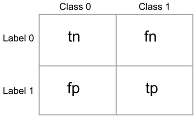
Figure 7: Estimated confusion matrix. The notation tp stands for "number of true positives", fn for "number of false negatives", and so on.

The rows correspond to class labels, the columns to true classes. We then have the following approximations:

$\begin{aligned} \mbox{Prevalence :} & \quad \pi_{1} &&\equiv\pi(\lambda_{1}) &&\approx \dfrac{\rm fn+tp}{\rm fn+tp+fp+tn}\\[1mm] \mbox{Queue rate :} & \quad p_{1} &&\equiv p(\ell_{1}) &&\approx \dfrac{\rm fp+tp}{\rm fn+tp+fp+tn}\\[4mm] \mbox{True-positive rate, sensitivity, recall :} & \quad S_{e} &&\equiv p(\ell_{1}\mid\lambda_{1}) &&\approx \dfrac{\rm tp}{\rm tp+fn}\\[1mm] \mbox{True-negative rate, specificity :} & \quad S_{p} &&\equiv p(\ell_{0}\mid\lambda_{0}) &&\approx \dfrac{\rm tn}{\rm tn + fp}\\[1mm] \mbox{False-positive rate, Type-I error rate :} & \quad \alpha &&\equiv p(\ell_{1}\mid\lambda_{0})&&\approx \dfrac{\rm fp}{\rm tn + fp}\\[1mm] \mbox{False-negative rate, Type-II error rate :} & \quad \beta &&\equiv p(\ell_{0}\mid\lambda_{1})&&\approx \dfrac{\rm fn}{\rm tp + fn}\\[4mm] \mbox{Positive predictive value, precision :} & \quad \mathit{ppv} &&\equiv p(\lambda_{1}\mid\ell_{1}) &&\approx \dfrac{\rm tp}{\rm tp + fp}\\[1mm] \mbox{Negative predictive value :} & \quad \mathit{npv} &&\equiv p(\lambda_{0}\mid\ell_{0}) &&\approx \dfrac{\rm tn}{\rm tn + fn}\\[1mm] \mbox{False-discovery rate :} & \quad \mathit{fdr} &&\equiv p(\lambda_{0}\mid\ell_{1}) &&\approx \dfrac{\rm fp}{\rm tp + fp}\\[1mm] \mbox{False-omission rate :} & \quad \mathit{for} &&\equiv p(\lambda_{1}\mid\ell_{0}) &&\approx \dfrac{\rm fn}{\rm tn + fn}\\[4mm] \mbox{Positive likelihood ratio :} & \quad {\rm lr+} &&\equiv \frac{p(\ell_{1}\mid\lambda_{1})}{p(\ell_{1}\mid\lambda_{0})}&&\approx \frac{\rm tp}{\rm tp+fn}\; \frac{\rm tn+fp}{\rm fp}\\[1mm] \mbox{Negative likelihood ratio :} & \quad {\rm lr-} &&\equiv \frac{p(\ell_{0}\mid\lambda_{1})}{p(\ell_{0}\mid\lambda_{0})}&&\approx \frac{\rm fn}{\rm tp+fn}\; \frac{\rm tn+fp}{\rm tn}\\[1mm] \mbox{Diagnostic odds ratio :} & \quad \mathit{dor} &&\equiv \frac{\rm lr+}{\rm lr-} &&\approx \frac{\rm tp}{\rm fp} \frac{\rm tn}{\rm fn}\\[4mm] \mbox{Accuracy :} & \quad A &&\equiv p(\ell=\lambda) &&\approx \dfrac{\rm tp + tn}{\rm tp + tn + fp + fn} \end{aligned}$

There are no simple expressions for the AUROC and AUPRC, since these require integration under the ROC and PRC, respectively.

Note that the relations between probabilities derived in the previous sections also hold between their estimates.

9. Trends and baselines

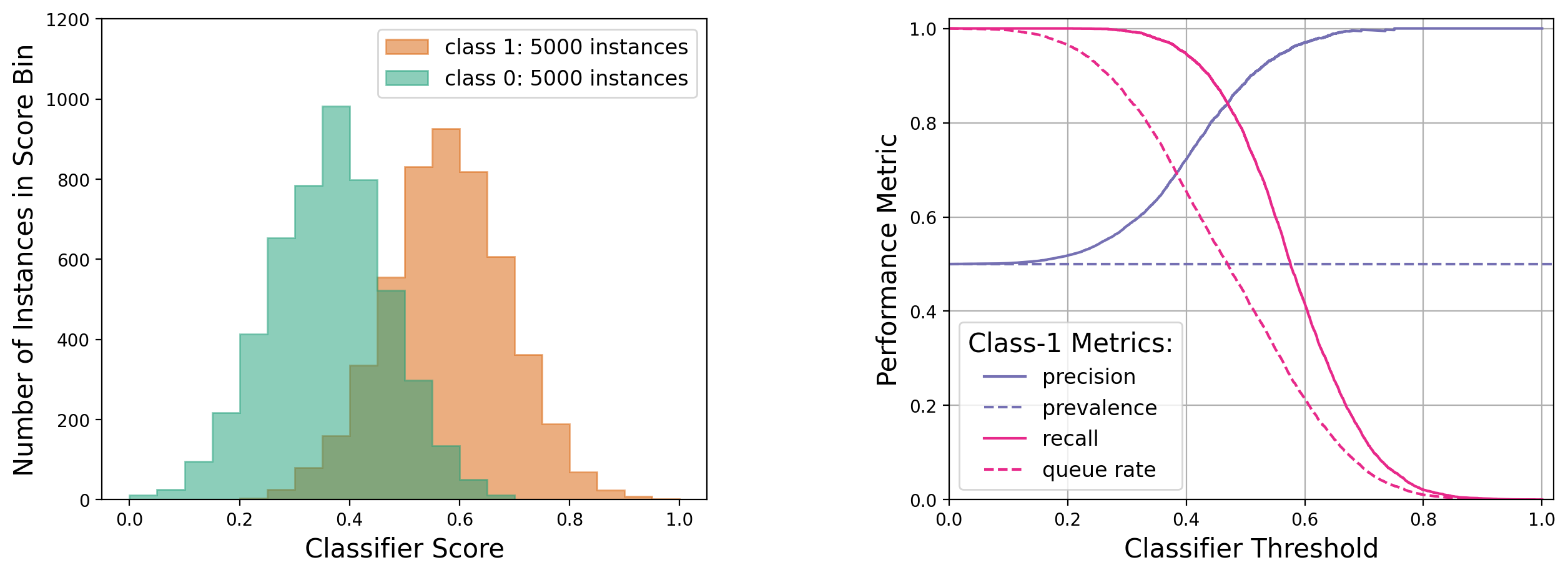
For classifiers that generate scores it is useful to understand how various metrics change as the classifier threshold on the score is increased. This will of course depend on the actual score distributions of true class-0 and true class-1 instances. In the following four illustrations we keep these two distributions identical: one a Gaussian with mean 0.25 and width 0.25, and the other a Gaussian with mean 0.75 and width 0.25. What changes is the sample composition: balanced or imbalanced, high- or low-statistics; and which class is represented by which Gaussian.

Case 1: Balanced, high-statistics dataset, with class-1 scores mostly above class-0 scores

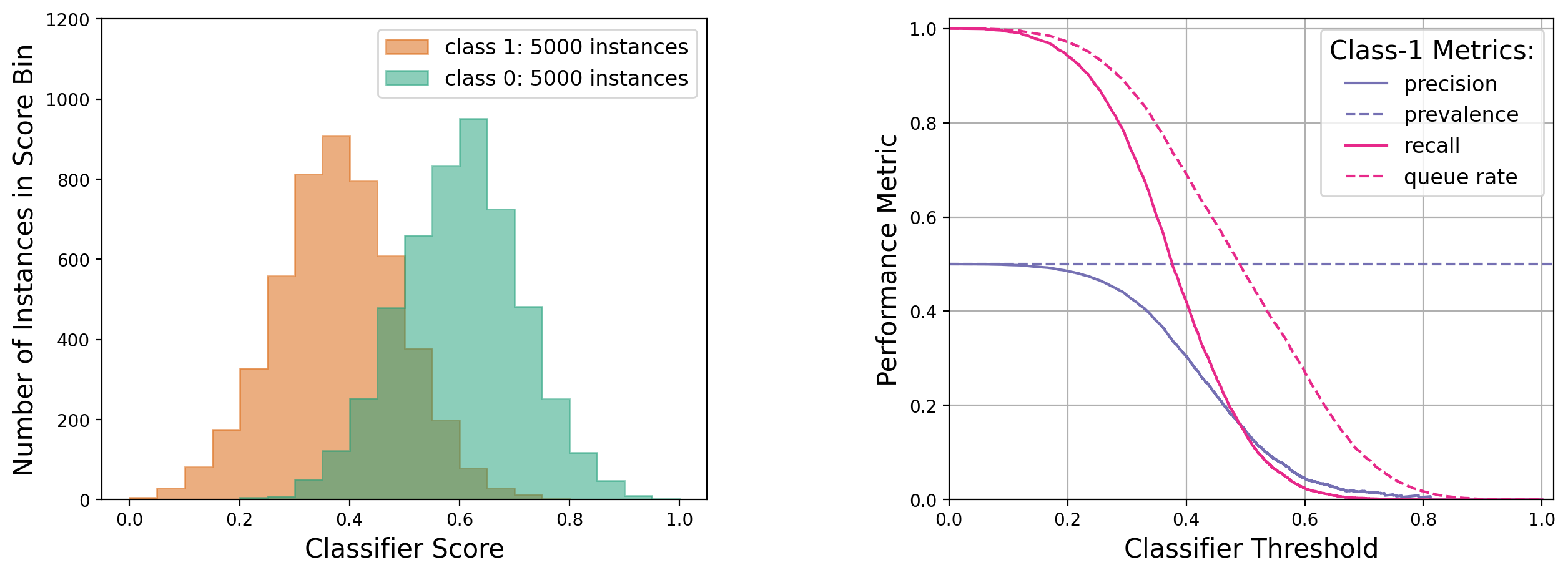
Figure 8. The recall and queue rate both decrease, whereas the precision increases. As noted previously, if the classifier threshold is chosen such that queue rate equals prevalence, precision will equal recall.

Case 2: Balanced, high-statistics dataset, with class-1 scores mostly below class-0 scores

Figure 9. Compared to Case 1 the recall is still decreasing with threshold, but the precision is now decreasing instead of increasing. The baselines are now *above* their corresponding metrics, indicating that the classifier is misleading.

Case 3: Balanced, low-statistics dataset, with class-1 scores mostly above class-0 scores

Figure 10. The curves are essentially the same as for Case 1, but with pronounced statistical fluctuations. Note that the recall never fluctuates up: it stays even or decreases. In contrast, the precision fluctuates both up and down.

Case 4: Imbalanced, high-statistics dataset, with class-1 scores mostly above class-0 scores

Figure 11. Compared to Case 1, the recall hasn't changed, but its baseline, the queue rate, has shifted down as a whole. The precision has also shifted down.

See appendix 11.2 for a more detailed explanation of the above trends.

10. Effect of prevalence on classifier training and testing

In this post I have tried to be careful in pointing out which performance metrics depend on the prevalence, and which don’t. The reason is that prevalence is a population or sample property, whereas here we are interested in classifier properties. Of course, real-world classifiers must be trained and tested on finite samples, and this has implications for the actual effect of prevalence on classifier performance:

When training a classifier, changing the prevalence in the training data may affect properties such as the sensitivity and specificity, depending on the characteristics of the training algorithm.
When testing a trained classifier, changing the prevalence in the test data will not affect properties such as the sensitivity and specificity (within statistical fluctuations).

To illustrate this point I went back to a previous post on predicting flight delays with a random forest. The prevalence of the given flight delay data set is about 20%, but can be increased by randomly dropping class 0 instances (non-delayed flights). The table below shows the effect of changing the prevalence in this way in the training data:

Training set prevalence	Sensitivity	Specificity	Accuracy	AUROC
0.40	0.16	0.96	0.72	0.72
0.42	0.29	0.91	0.72	0.72
0.44	0.46	0.82	0.71	0.72
0.46	0.58	0.72	0.68	0.71
0.48	0.63	0.67	0.66	0.72
0.50	0.73	0.57	0.62	0.71

To be clear, for each row it is the same classifier (same hyper-parameters: number of trees, maximum tree depth, etc.) that is being fit to a training data set with varying prevalence. The sensitivity, specificity, accuracy, and AUROC are then measured on a testing data set with a constant prevalence of 30%. Note how the sensitivity and specificity, as measured on an independent test data set, vary with training set prevalence. The AUROC, on the other hand, remains stable.

Next, let’s look at the effect of changing the prevalence in the testing data:

Testing set prevalence	Sensitivity	Specificity	Accuracy	AUROC
0.20	0.50	0.78	0.73	0.72
0.30	0.48	0.80	0.70	0.72
0.40	0.45	0.82	0.67	0.72
0.50	0.46	0.80	0.63	0.71
0.60	0.50	0.79	0.61	0.71

Here the prevalence in the training data was set at 0.45. The sensitivity and specificity appear much more stable; residual variations may be due to the effect on the training data set of the procedure used to vary the testing set prevalence.

Training data sets are often unbalanced, with prevalences even lower than in the example discussed here. Modules such as scikit-learn’s RandomForestClassifier provide a class_weight option, which can be set to balanced or balanced_subsample in order to assign a larger weight to the minority class. This re-weighting is applied both to the GINI criterion used for finding splits at decision tree nodes and to class votes in the terminal nodes. The sensitivity and specificity of a classifier, as well as its accuracy, will depend on the setting of the class_weight option. For scoring purposes when optimizing a classifier, AUROC tends to be a much more robust property.

11. Mathematical Appendix

This appendix contains mathematical proofs of some of the statements made in the body of this post.

11.1 Expectation values of sensitivity, specificity, and accuracy

To see how the AUROC is related to an expectation value of the sensitivity, note that for a given threshold $q_{T}$ on the classifier output score, we can write the sensitivity as:

$S_{e}(q_{T}) \;=\; \mathbb{P}\left[Q_{1}\ge q_{T}\right],$

where $Q_{1}$ is a random variable distributed as the classifier scores of positive instances. Let us now compute the expectation value of $S_{e}(q_{T})$ where $q_{T}$ is varied over the distribution of classifier scores of all instances in the population of interest, class 0 and class 1. This score distribution can be modeled by a random variable $Q^{\prime}$ defined as follows:

$Q^{\prime} \;\equiv\; \mathbb{1}(U \le \pi_{0})\, Q^{\prime}_{0} \;+\; \mathbb{1}(U \gt \pi_{0})\, Q^{\prime}_{1},$

where $\mathbb{1}(A)$ is the indicator function of set $A$ , and $U$ , $Q^{\prime}_{0}$ and $Q^{\prime}_{1}$ are independent random variables, with $U$ being uniform between 0 and 1, and $Q^{\prime}_{0}$ , $Q^{\prime}_{1}$ following the score distributions of class-0, resp. class-1 instances. Extending the definition of $S_{e}$ to a function of a random threshold:

$S_{e}(Q^{\prime}) \;\equiv\; \mathbb{P}\left[Q_{1} \ge Q^{\prime}\mid Q^{\prime}\right] \; = \; \mathbb{E}\left[\mathbb{1}(Q_{1} \ge Q^{\prime}) \mid Q^{\prime}\right],$

we then have:

$\begin{align} \mathbb{E}\left[S_{e}\right] \;&\equiv\; \mathbb{E}\left[ \;\mathbb{E}\left[ \mathbb{1}(Q_{1} \ge Q^{\prime})\mid Q^{\prime} \right]\; \right]\\[1mm] \;&=\; \mathbb{E}\left[ \mathbb{1}(Q_{1} \ge Q^{\prime})\right]\quad\textrm{by the law of total expectation,}\\[1mm] \;&=\; \mathbb{E}\left[ \mathbb{1}(U \le \pi_{0})\;\mathbb{1}(Q_{1} \ge Q^{\prime}_{0}) \;+\; \mathbb{1}(U > \pi_{0})\;\mathbb{1}(Q_{1} \ge Q^{\prime}_{1}) \right]\quad\textrm{by definition of $Q^{\prime}$,}\\[1mm] \;&=\; \mathbb{E}\left[ \mathbb{1}(U \le \pi_{0})\;\mathbb{1}(Q_{1} \ge Q^{\prime}_{0})\right] \;+\; \mathbb{E}\left[ \mathbb{1}(U > \pi_{0})\;\mathbb{1}(Q_{1} \ge Q^{\prime}_{1}) \right]\quad\textrm{by linearity of the expectation operator,}\\[1mm] \;&=\; \mathbb{E}\left[ \mathbb{1}(U \le \pi_{0})\right] \; \mathbb{E}\left[ \mathbb{1}(Q_{1} \ge Q^{\prime}_{0})\right] \;+\; \mathbb{E}\left[ \mathbb{1}(U > \pi_{0})\right] \; \mathbb{E}\left[ \mathbb{1}(Q_{1} \ge Q^{\prime}_{1}) \right]\quad\textrm{by independence of $U$, $Q_{1}$, $Q_{0}^{\prime}$, $Q_{1}^{\prime}$,}\\[1mm] \;&=\; \pi_{0}\,\mathbb{P}\left(Q_{1} \ge Q^{\prime}_{0}\right) \;+\; \pi_{1}\,\mathbb{P}\left(Q_{1} \ge Q^{\prime}_{1}\right)\quad\textrm{by definition of $\mathbb{P}$ in terms of $\mathbb{E}$,}\\[1mm] \;&=\; \pi_{0}\, \textrm{AUROC} \;+\; \frac{\pi_{1}}{2}\quad\textrm{by definition of AUROC.} \end{align}$

One can similarly show that:

$\mathbb{E}\left[S_{p}\right] \;=\; \pi_{1}\, \textrm{AUROC} \;+\; \frac{\pi_{0}}{2}.$

Using the expression for the accuracy A in terms of $S_{e}$ and $S_{p}$ , and the linearity of the expectation operator, we then find:

$\mathbb{E}\left[A\right] \;=\; 2\,\pi_{0}\,\pi_{1}\,\textrm{AUROC} \,+\, \frac{\pi_{0}^{2} + \pi_{1}^{2}}{2}.$

11.2 Performance metrics versus threshold

To understand the behavior of the performance metrics in section 9, consider what happens when we increase the classifier threshold $t$ by an amount $\Delta t \gt 0$ . A number $\Delta p + \Delta n$ of instances will see their labels flip from 1 to 0, where $\Delta p$ are class-1 and $\Delta n$ are class-0. The effect on the confusion matrix elements is:

$\begin{align*} {\rm tp} &\quad\longrightarrow\quad {\rm tp} - \Delta p\\ {\rm fn} &\quad\longrightarrow\quad {\rm fn} + \Delta p\\ {\rm tn} &\quad\longrightarrow\quad {\rm tn} + \Delta n\\ {\rm fp} &\quad\longrightarrow\quad {\rm fp} - \Delta n \end{align*}$

Applying these transformations to the metrics in section 8 yields the following results.

For the queue rates:

$\begin{align*} p_{1} &= \frac{\rm tp+fp}{\rm tn+fn+tp+fp} \quad\longrightarrow\quad p_{1} \;-\; \frac{\Delta p + \Delta n}{\rm tn+fn+tp+fp}\\ p_{0} &= \frac{\rm tn+fn}{\rm tn+fn+tp+fp} \quad\longrightarrow\quad p_{0} \;+\; \frac{\Delta p + \Delta n}{\rm tn+fn+tp+fp} \end{align*}$

For the likelihoods:

$\begin{align*} S_{e} &= \frac{\rm tp}{\rm tp+fn} \quad\longrightarrow\quad S_{e}\;-\; \frac{\Delta p}{\rm tp + fn}\\ \beta &= \frac{\rm fn}{\rm tp+fn} \quad\longrightarrow\quad \beta\;+\; \frac{\Delta p}{\rm tp + fn}\\ S_{p} &= \frac{\rm tn}{\rm tn+fp} \quad\longrightarrow\quad S_{p}\;+\; \frac{\Delta n}{\rm tn + fp}\\ \alpha &= \frac{\rm fp}{\rm tn+fp} \quad\longrightarrow\quad \alpha\;-\; \frac{\Delta n}{\rm tn + fp} \end{align*}$

Note in particular how the recall $S_{e}$ and class-1 queue rate $p_{1}$ always decrease when the threshold is increased, explaining the behavior in the graphs. However the change in predictive values is not linear. For the class-1 precision for example, we have:

$\mathit{ppv} = \frac{\rm tp}{\rm tp+fp} \quad\longrightarrow\quad \frac{ {\rm tp} - \Delta p}{ {\rm tp} - \Delta p + {\rm fp} - \Delta n},$

so that $\mathit{ppv}$ will increase if and only if:

$\frac{\Delta p}{\rm tp} \; <\; \frac{\Delta n}{\rm fp},$

i.e., if the fractional loss of true positives is smaller than the fractional loss of false positives. This inequality can be violated “locally” by statistical fluctuations (Case 3 in section 9), or “globally”, when the class-0 score distribution is on the wrong side of the class-1 score distribution (Case 2 in section 9).